1 Sampling Workflow
The goal of statistical audit sampling is to infer the misstatement in a population based on a representative sample. This can be challenging, but the Audit module simplifies the process into four stages: planning, selection, execution, and evaluation.

More detailed information about the individual stages in the audit sampling workflow is provided below.
1.1 The four stages of the sampling workflow
In the planning stage, you determine the sample size needed to support the assertion that the population’s misstatement is below the performance materiality. This involves using prior audit outcomes and information about inherent risk and control risk. Expectations about error rates also influence the sample size required to maintain statistical confidence.
Using the sample size from the planning stage, you select a statistically representative sample. Each sampling unit receives an inclusion probability, and units are selected based on these probabilities. Monetary unit sampling assigns probabilities to individual monetary units, making higher-value items more likely to be selected. Record sampling assigns equal probabilities to all items.
In the execution stage, you assess the correctness of selected items. The simplest method categorizes items as correct or incorrect, while a more accurate method considers the true value (audit value) of items. Annotating samples with audit values provides a more precise estimate of misstatement. If book values are unavailable, use the correct/incorrect method.
In the evaluation stage, you use the annotated sample to infer the total misstatement in the population. Statistical techniques calculate a projected maximum misstatement, and the population is approved if this is below the performance materiality.
This manual emphasizes the practical application of the audit sampling workflow in JASP. For a deeper understanding of the statistical theory behind the four stages of the audit sampling workflow, read the free online book Statistical Audit Sampling with R.
1.2 Practical example
The Audit module in JASP offers two ways to navigate the audit sampling workflow: the Sampling Workflow analysis, which guides you through all four stages, and individual analyses for Planning, Selection, and Evaluation. This chapter uses the classical sampling workflow analysis to explain the Audit module’s core functionality. Note that a Bayesian variant of the sampling workflow is also available.
Let’s explore an example of the audit sampling workflow. To follow along, open the ‘Testing for Overstatements’ dataset from the Data Library. Navigate to the top-left menu, click ‘Open’, then ‘Data Library’, select ‘7. Audit’, and finally click on the text ‘Testing for Overstatements’ (not the green JASP-icon button).
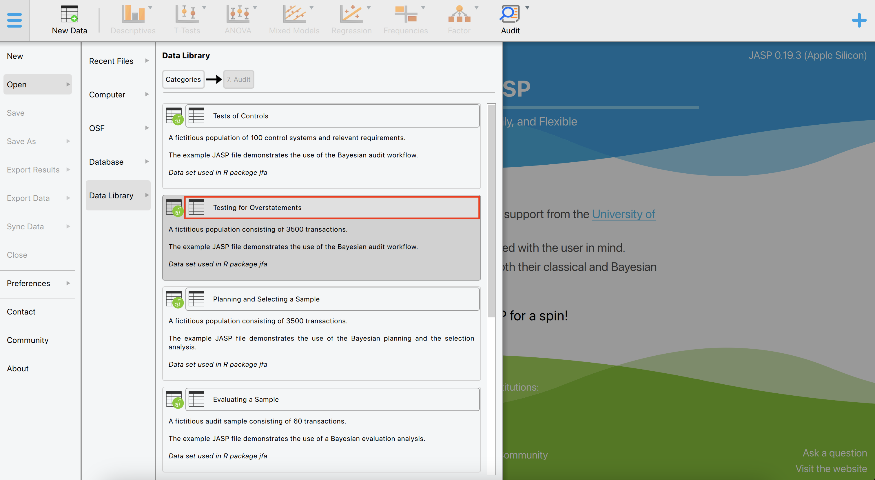
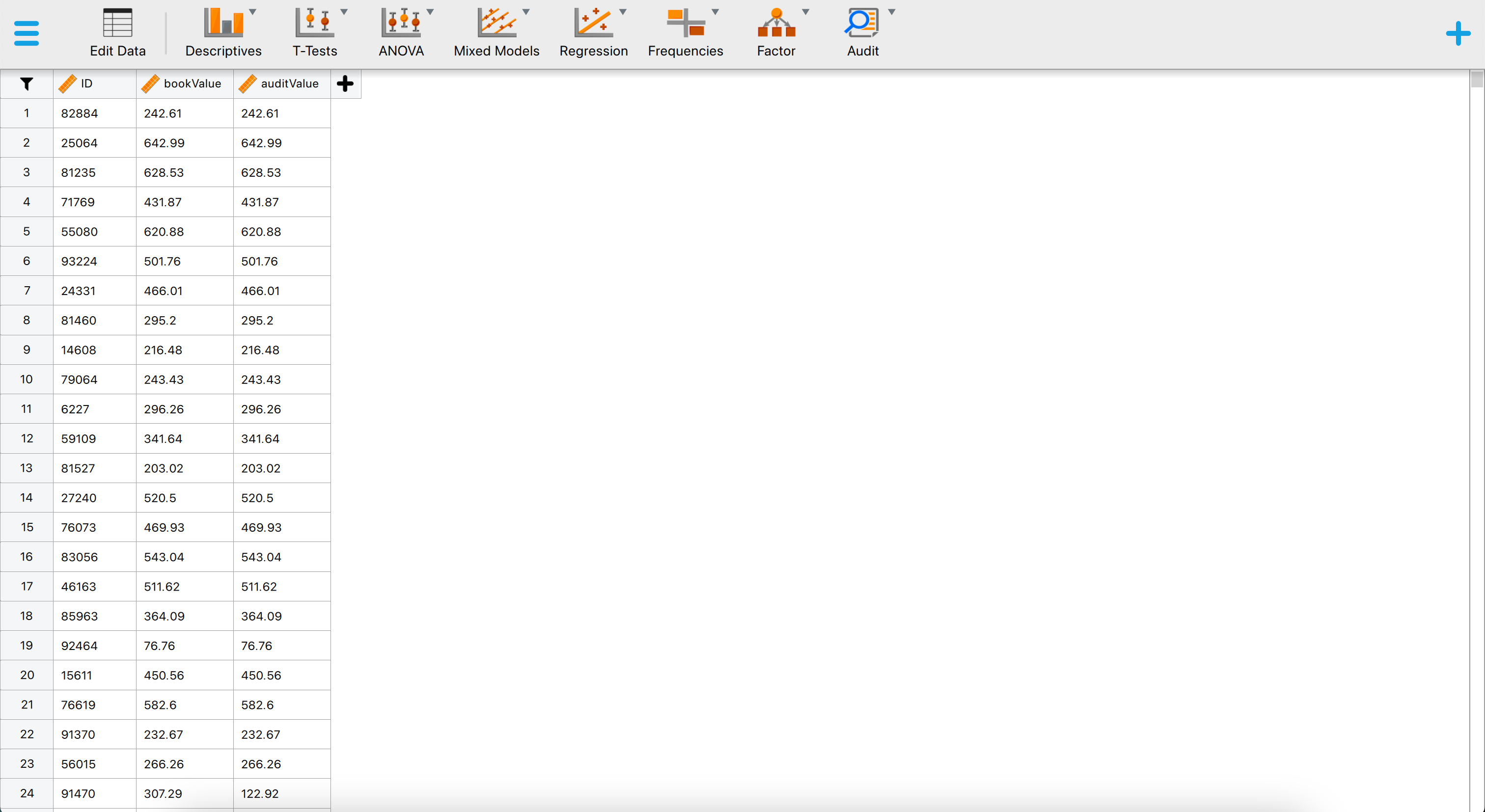
This will open a dataset with 3500 rows and three columns: ‘ID’, ‘bookValue’, and ‘auditValue’. The ‘ID’ column represents the identification number of the items in the population. The ‘bookValue’ column shows the recorded values of the items, while the ‘auditValue’ column displays the true values. The ‘auditValue’ column is included for illustrative purposes, as auditors typically know the true values only for the audited sample, not for all items in the population.
1.2.1 Stage 1: Planning
To start the sampling workflow, click on the Audit module icon and select ‘Sampling Workflow’. This will open the following interface, where you need to specify the settings for the statistical analysis.
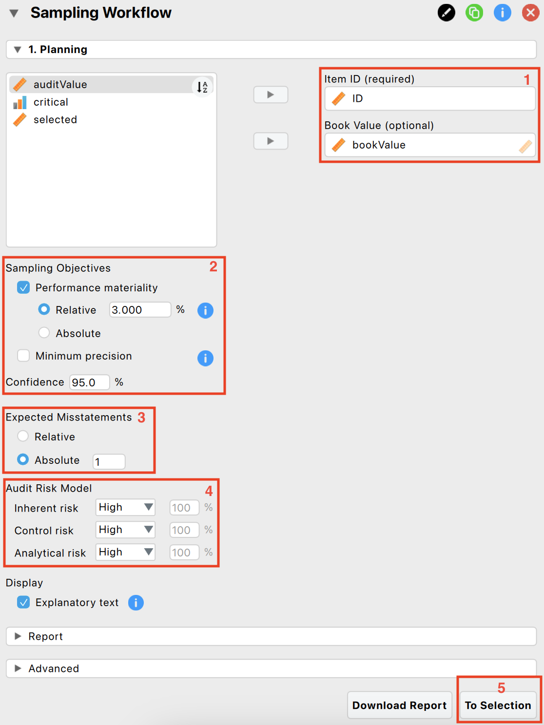
The following five settings are required:
Indicate the variables: First, enter the variable indicating the identification numbers of the items in the corresponding box. Optionally, if you have access to the book values of the items, you can enter this variable as well.
Sampling objectives: Next, formulate your sampling objectives. Enable the ‘Performance materiality’ objective if you want to test whether the total misstatement in the population exceeds a certain limit (i.e., the performance materiality). This approach enables you to plan a sample such that, when the sample meets your expectations, the maximum error is said to be below performance materiality. Enable the ‘Minimum precision’ objective if you want to obtain a required minimum precision when estimating the total misstatement in the population. This approach enables you to plan a sample such that, when the sample meets expectations, the uncertainty of your estimate is within a tolerable percentage. In the example, we choose a performance materiality of 3.5%.
Expected misstatement: Then, indicate how many misstatements are tolerable in the sample. In the example, we choose to tolerate one full misstatement in the sample.
Prior information: Additionally, indicate the risks of material misstatement via the audit risk model. According to the Audit Risk Model, audit risk can be divided into three constituents: inherent risk, control risk, and detection risk. Inherent risk is the risk posed by an error in a financial statement due to a factor other than a failure of internal controls. Control risk is the probability that a material misstatement is not prevented or detected by the internal control systems of the company (e.g., computer-managed databases). Both these risks are commonly assessed by the auditor on a 3-point scale consisting of low, medium, and high. Detection risk is the probability that an auditor will fail to find material misstatements in an organization’s financial statements. For a given level of audit risk, the tolerable level of detection risk bears an inverse relationship to the other two assessed risks. Intuitively, a greater risk of material misstatement should require a lower tolerable detection risk and, accordingly, more persuasive audit evidence. In this example, we choose to set all risks to ‘High’ and solely rely on evidence from substantive testing.
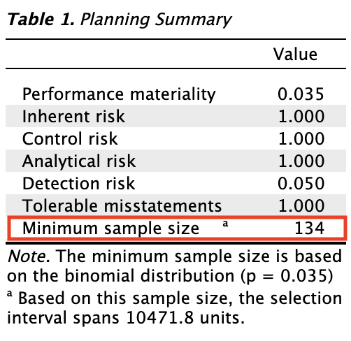
The primary output from the planning stage, shown below, indicates that a minimum sample size of 134 sampling units is required to achieve 95% assurance that the misstatement in the population is below 3.5%, while allowing for one misstatement in the sample.
- Next stage: Finally, progress to the selection stage by clicking the ‘To Selection’ button.
For a more detailed explanation of the settings and output in the planning stage, see Chapter 2.
1.2.2 Stage 2: Selection
In the selection stage, you must select the 134 sampling units from the population. Once the ‘To Selection’ button is pressed, the interface from the selection stage opens.
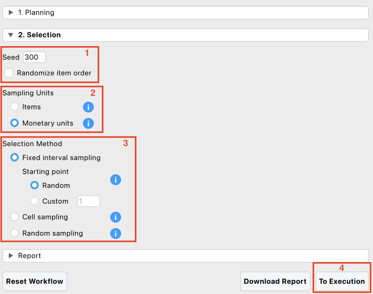
The following four settings are required:
Randomness: Begin by selecting the settings related to randomness in the selection procedure. The seed setting is important as it ensures that random procedures are reproducible, allowing for consistent results across multiple runs. A random number will be chosen each time you start the analysis. Additionally, the ‘Randomize item order’ setting is available to randomly shuffle the rows in the dataset, which can help mitigate any biases that might arise from the original order of the data.
Sampling units: Next, specify the sampling units for the selection process. These units can either be items or monetary units. If no book value variable is provided, the sampling units default to ‘Items’, enabling attribute sampling. Conversely, if a book value variable was indicated during the planning stage, the sampling units default to ‘Monetary units’, facilitating monetary unit sampling (MUS). MUS is particularly useful for auditing financial data as it considers the monetary value of each unit.
Sampling method: Then, choose the selection method to be used in the sampling process. The available algorithms include:
- Fixed interval sampling: This method selects units at regular intervals from the dataset, ensuring a systematic sampling approach.
- Cell sampling: This technique involves dividing the dataset into cells and randomly selecting units from each cell, promoting a systematic sampling approach with a bit of randomness.
- Random sampling: This approach randomly selects units from the entire dataset, providing a simple yet effective method for ensuring randomness.
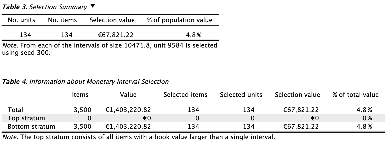
The primary output from the selection stage, as shown in the first table below, reveals that 134 sampling units were selected from 134 items. The sample’s total value amounts to €67,821.22, representing 4.8% of the total population value. The second table provides details specific to interval selection using monetary unit sampling. It indicates the number of items selected in the ‘Top stratum’, which includes all items larger than a single interval (for fixed interval selection). In this instance, there were 0 items in the top stratum.
- Next stage: Finally, progress to the execution stage by clicking the ‘To Execution’ button.
1.2.3 Stage 3: Execution
In the execution stage, you must judge the fairness of the 134 sampled items. Once the ‘To Execution’ button is pressed, the interface from the execution stage opens.
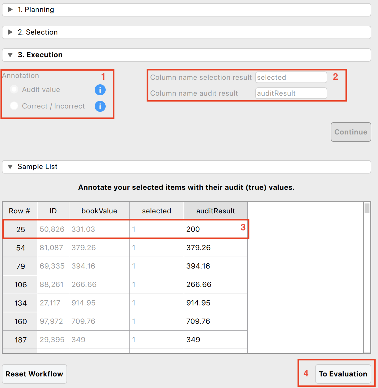
The following four settings are required:
Annotation method: First, decide how to annotate the selected items. You have two choices:
- Audit value: Annotate the items with their audit (true) values. This method is recommended (and automatically selected) when the items have a monetary value.
- Correct / Incorrect: Annotate the items as correct (0) or incorrect (1). This method is recommended (and automatically selected) when the items do not have a monetary value.
Column names: Next, specify the names of the two columns that will be added to the dataset. The first column name will indicate the result of the selection, while the second column name will contain the annotation of the items. Click the ‘Continue’ button to confirm the settings and open the data viewer.
Annotating items: Then, use the data viewer to annotate the selected items with their book value. For example, in this case, item 50826 (row 25, highlighted in red) had a book value of €333.03 but a true value of €200. The remaining items have correctly reported book values.
Next stage: Finally, progress to the evaluation stage by clicking the ‘To Evaluation’ button.
1.2.4 Stage 4: Evaluation
In the evaluation stage, you assess the misstatement in the sample and extrapolate it to the entire population. Once you press the ‘To Evaluation’ button, the interface for the evaluation stage will open.
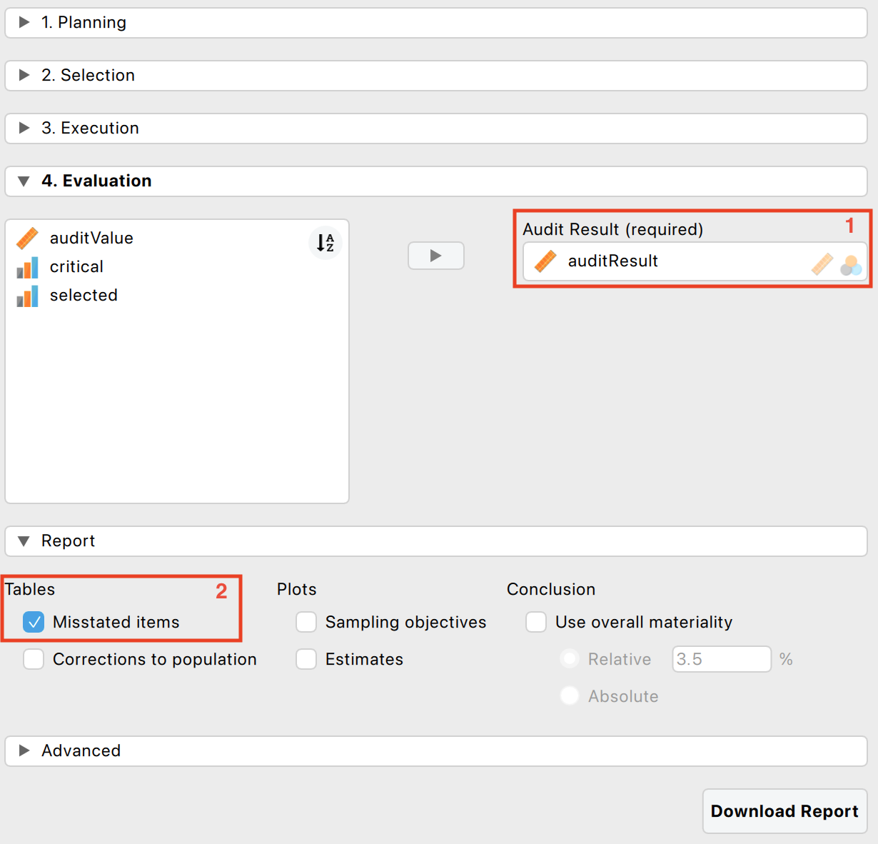
The following setting is required:
- Annotation variable: Specify the variable that contains the annotation of the items in the corresponding box.
The following setting is optional:
- Additional tables: It is recommended to request the ‘Misstated items’ table from the ‘Report’ section. This table displays the items in the sample where the book value did not match the true value. Additional tables and figures to clarify the output, which will be discussed in Chapter 4, can be requested here as well.
The primary output from the evaluation stage, as shown in the first table below, indicates that the most likely misstatement in the population is estimated to be 0.003, or 0.3%. The 95% upper bound for this estimate is 0.027, or 2.7%. This upper bound is lower than the performance materiality of 3.5%, meaning the auditor has achieved at least 95% assurance that the population misstatement is below the performance materiality.
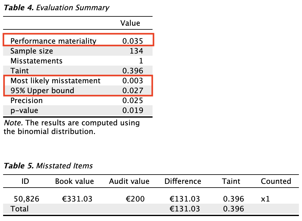
Based on the results of this statistical analysis, the auditor concludes that the population is free of material misstatement.