7 Benford’s Law
This chapter is about the ‘Benford’s Law’ analysis in the ‘Data Auditing’ section of the module.
7.1 Purpose of the analysis
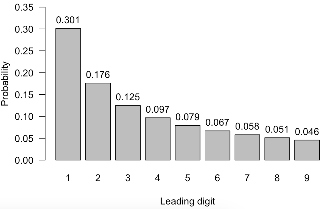
Benford’s law states that the distribution of leading digits in a population naturally follows a certain distribution. Specifically, the frequencies of each leading digit d are defined by p(d) = log\(_{10}\)(1 + \(\frac{1}{d}\)), see the figure below. For instance, the probablity of observing a 1 as a leading digit is 0.301, or 30.1%. This can be tested in a statistical manner. That is, the null hypothesis, H\(_0\), states that the distribution of first digits follows Benford’s law, while the alternative hypothesis, H\(_1\), states that it does not.
The purpose of the analysis in JASP is to investigate whether the distribution of first, second, or last digits in a set of numbers follows Benford’s law. In auditing, this may provide evidence that certain items or transactions in a population might warrant further investigation.
7.2 Practical example
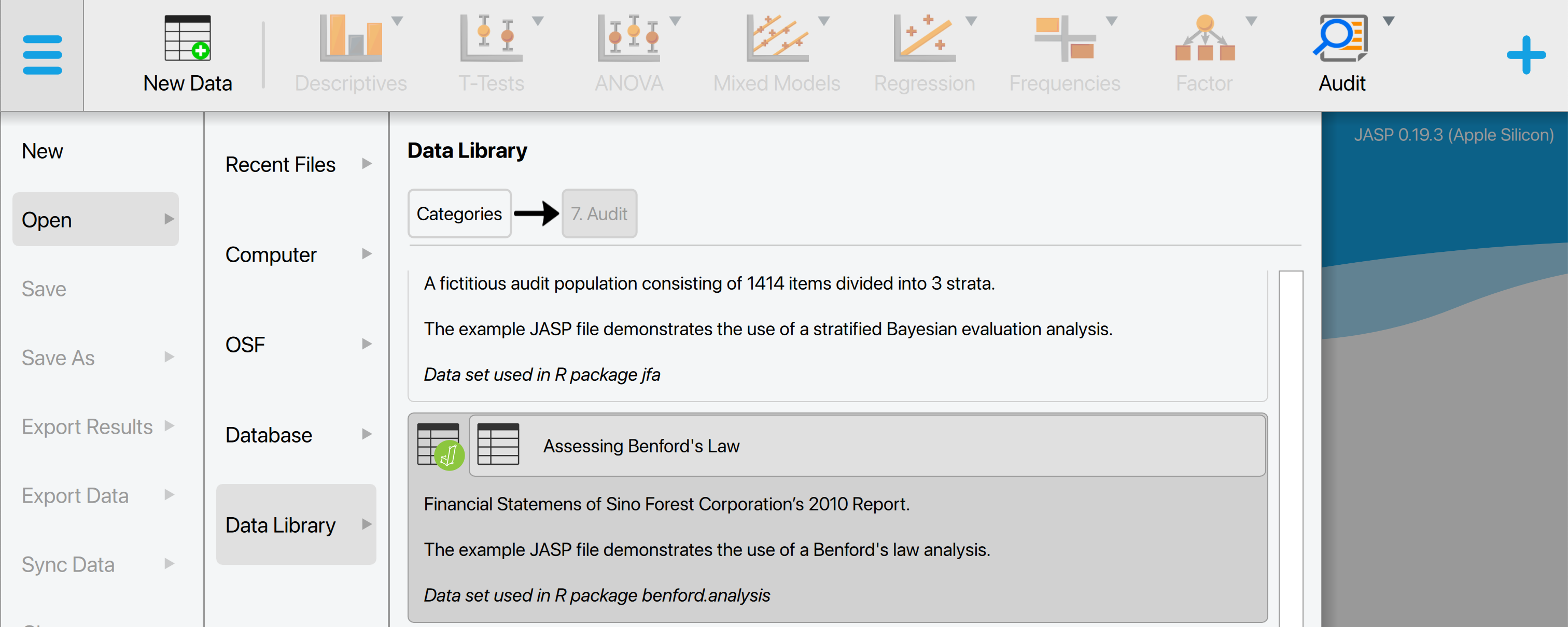
Let’s explore an example analysis of Benford’s law. To follow along, open the ‘Assessing Benford’s Law’ dataset from the Data Library. Navigate to the top-left menu, click ‘Open’, then ‘Data Library’, select ‘7. Audit’, and finally click on the text ‘Assessing Benford’s Law’ (not the green JASP-icon button).
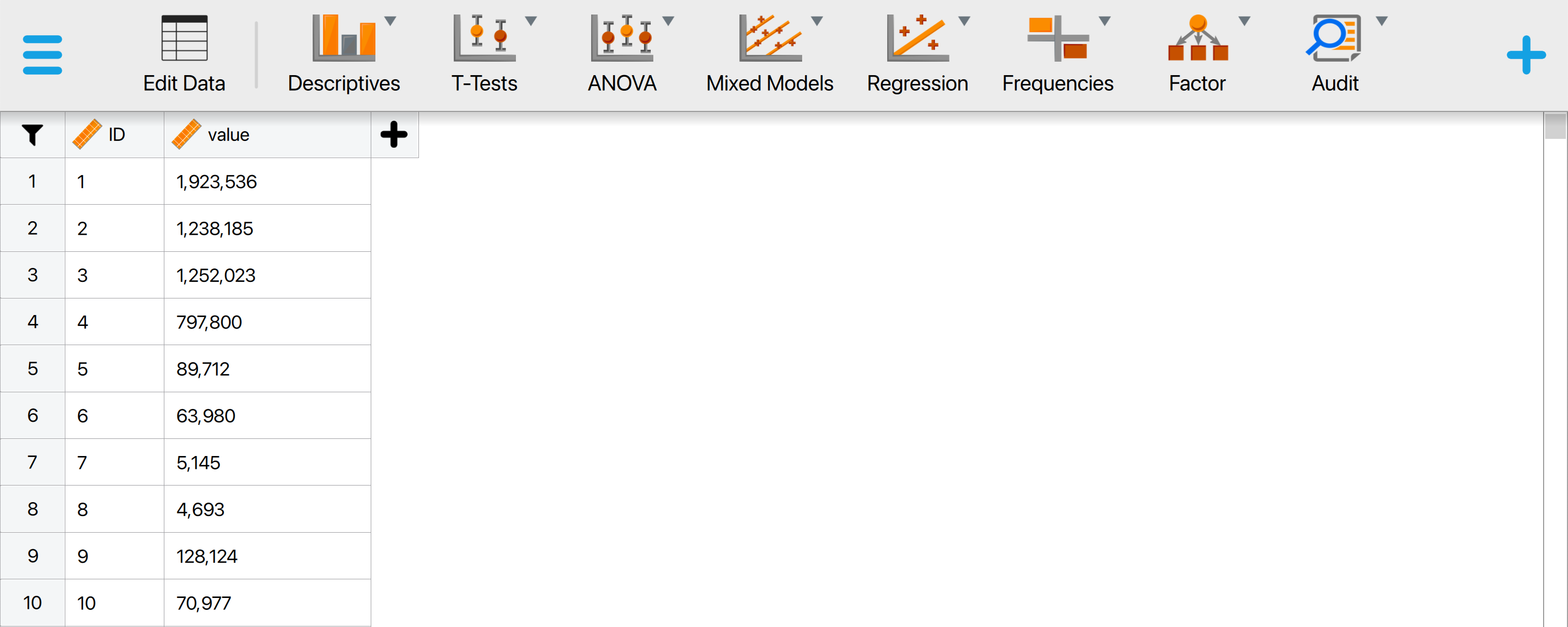
This will open a dataset with 772 rows and two columns: ‘ID’ and ‘value’. The ‘ID’ column represents the identification number of the items in the population. The ‘value’ column shows the recorded values of the items.
7.2.1 Main settings
In this example, we will investigate whether the distribution of first digits in the variable ‘value’, which represents the recorded values of transactions in a financial population, adheres to Benford’s law. That is, the null hypothesis, H\(_0\), states that the distribution of first digits follows Benford’s law, while the alternative hypothesis, H\(_1\), states that it does not. To test this, we open the ‘Benford’s Law’ analysis from the Audit module. The interface of the Benford’s law analysis is shown below.
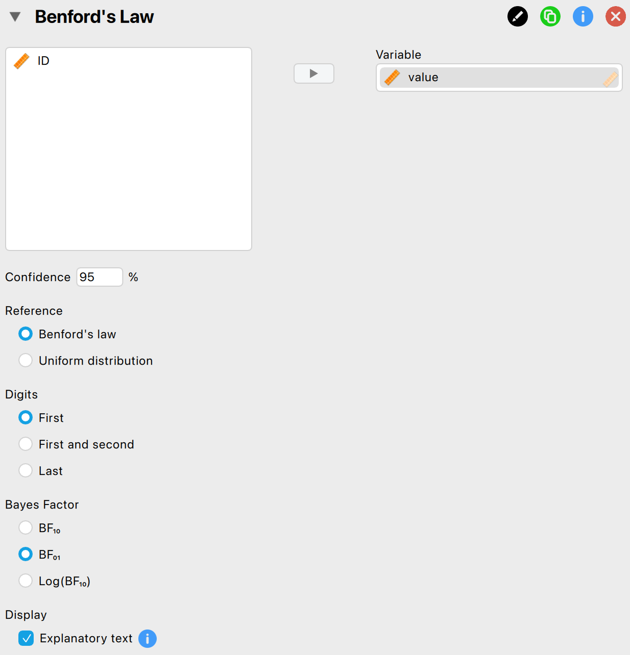
These are the main settings for the analysis:
- Variable: Begin by entering the variable whose digit distribution you wish to test in the designated box. In the example, this is the variable ‘value’, so we drag this variable to the field on the right.
- Confidence: Indicate the confidence level for your analysis. This level, which complements the significance level, determines when to reject the null hypothesis. In the example, we use a confidence level of 95%.
- Reference: Select a reference distribution to compare the chosen digits against. By default, this is set to ‘Benford’s law,’ but you can also opt for a uniform distribution. In the example, we select ‘Benford’s law’.
- Digits: Choose which digits to compare against the reference distribution. You can select the first digits (default), the first two digits, or the last digits. Benford’s law typically applies to the first or first two digits, while the uniform distribution is usually applied to the last digits. In the example, we choose to test the first digits against Benford’s law.
- Bayes factor: Select which Bayes factor is displayed in the main output table. ‘BF\(_{10}\)’ represents the Bayes factor in favor of the alternative hypothesis over the null hypothesis, ‘BF\(_{01}\)’ represents the Bayes factor in favor of the null hypothesis over the alternative hypothesis, and ‘Log(BF\(_{10}\))’ represents the logarithm of BF\(_{10}\).
- Display: Explanatory text: Finally, select whether to show explanatory text in the output.
7.2.2 Main output
The main table in the output, shown below, shows the sample size (n), the mean absolute deviation (MAD), the chi-square value (\(X^2\)) and its degrees of freedom (df). The table shows a p-value of 0.478, indicating that H\(_0\) should not be rejected at a significance level of 5%. Furthermore, the table presents the Bayes factor in favor of the null hypothesis, BF\(_{01}\), which is 6.9x10\(^6\). This suggests that the data provide very strong evidence supporting H\(_0\) over H\(_1\).
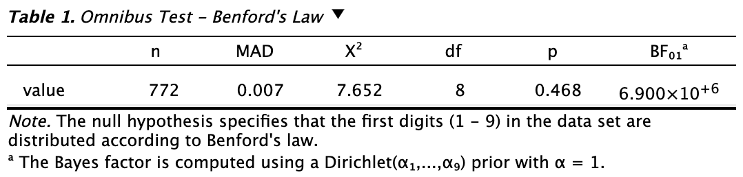
Note that non-conformity to Benford’s law does not necessarily indicate fraud. A Benford’s law analysis should therefore only be used to acquire insight into whether a population might need further investigation.
7.2.3 Report
The following settings enable you to expand the report with additional output, such as tables and figures.
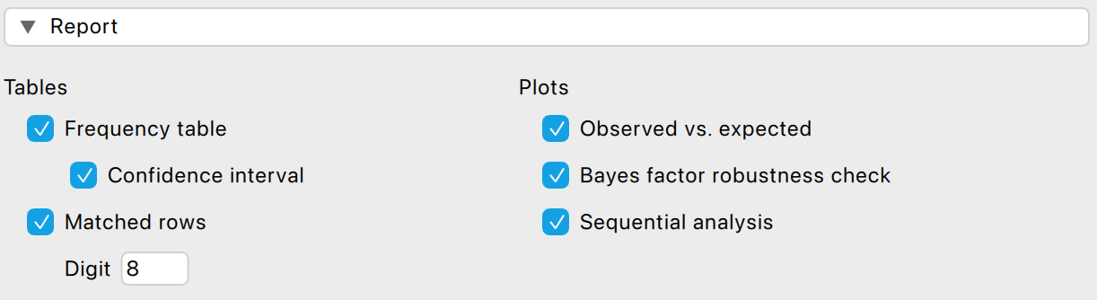
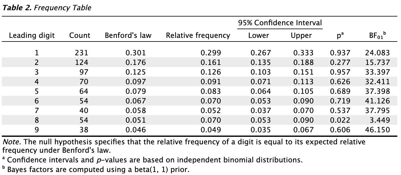
Tables: Frequency table: Check this box to display a table of the observed and expected frequencies of the digits. Clicking the ‘Confidence interval’ option shows confidence intervals for the observed relative frequencies in the table.
The frequency table displays the observed count for each leading digit in the second column. Adjacent to this, it shows the expected relative frequency under Benford’s law alongside the observed relative frequency in the data. Additionally, p-values and Bayes factors are provided to test whether the observed relative frequencies differ from the expected ones. In this case, only the digit 8 has a p-value smaller than 0.05, indicating a significant deviation from the expected relative frequency under Benford’s law.
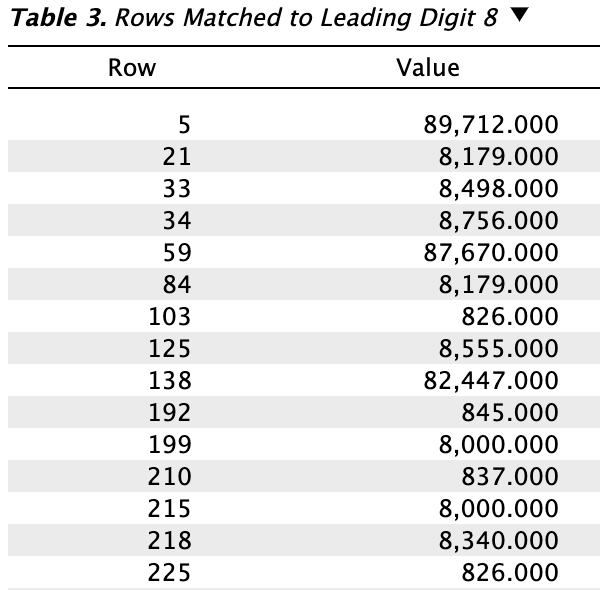
Tables: Matched rows: Check this box to display a table showing the rows that have a certain number as their leading/last digit(s).
In the example, we request a table of rows that match the digit 8. The first column displays the row number where the digit is found, and the second column shows the matched value. Using this table, you can identify the transactions that may warrant further investigation.
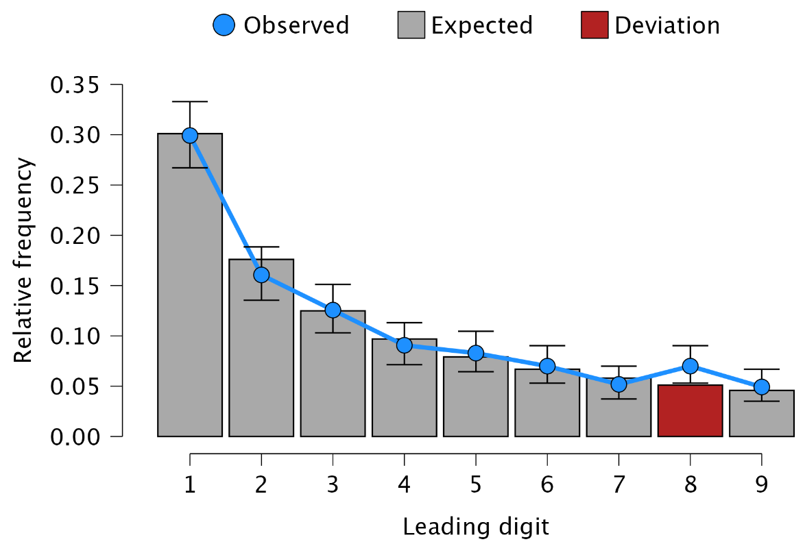
Plots: Observed vs. expected: Check this box to display a figure that illustrates the observed frequencies compared to the expected frequencies.
The figure in the output visualizes the observed relative frequencies compared to the expected ones, with the digit 8 highlighted in red. From this figure, it is immediately clear that the transactions starting with the digit 8 may warrant further inspection.
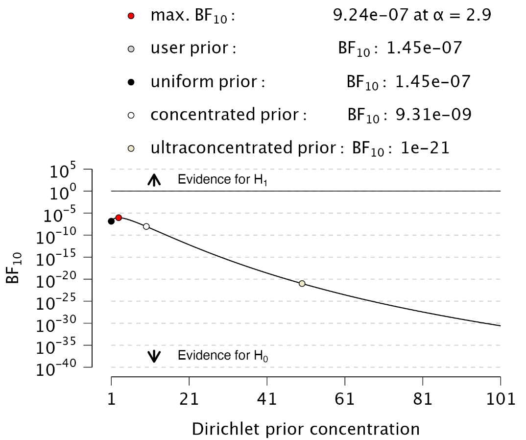
Plots: Bayes factor robustness check: Check this box to display a figure that shows the Bayes factor under different specifications of the prior concentration parameter.
The figure below is referred to as a robustness check. If the Bayes factor supports a particular hypothesis across all reasonable values of the prior concentration parameter, the result is considered robust regarding the choice of prior distribution. In this instance, the figure demonstrates that the Bayes factor consistently provides evidence in favor of the null hypothesis, regardless of the prior concentration parameter values.
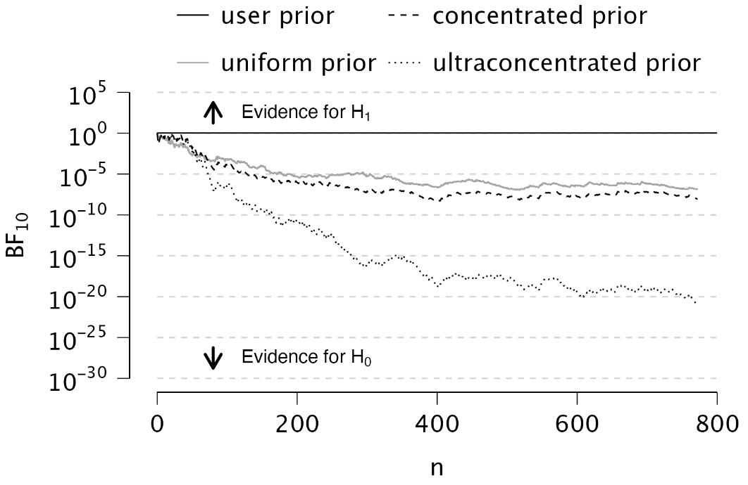
Plots: Sequential analysis: Select this box to display a figure illustrating the Bayes factor as a function of sample size, across various prior specifications.
In the example analysis, the sequential analysis plot demonstrates that the Bayes factor provides increasing evidence in favor of H\(_0\) as the sample size grows. Additionally, this evidence is more pronounced when using a more concentrated prior distribution.
7.2.4 Advanced
The following advanced settings enable you to customize the statistical computations according to your preferences.
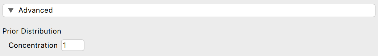
- Prior distribution: Concentration: Specify the concentration parameter for the Dirichlet prior distribution. Adjusting this value will alter the Bayes factor in the main output table. A larger concentration parameter indicates a more concentrated prior distribution, suggesting that the population proportions are more similar. When testing against the uniform distribution, this implies a stronger belief in H\(_0\). Conversely, when testing against Benford’s law, it indicates a stronger belief in H\(_1\).