Algorithmic fairness

Introduction

Welcome to the ‘Algorithmic fairness’ vignette of the jfa package. This page provides a comprehensive example of how to use the model_fairness() and the fairness_selection() functions in the package.

Function: `model_fairness()`

The model_fairness() function offers methods to evaluate fairness in algorithmic decision-making systems. It computes various model-agnostic metrics based on the observed and predicted labels in a dataset. The fairness metrics that can be calculated include demographic parity, proportional parity, predictive rate parity, accuracy parity, false negative rate parity, false positive rate parity, true positive rate parity, negative predicted value parity, and specificity parity (Calders & Verwer, 2010; Chouldechova, 2017; Feldman et al., 2015; Friedler et al., 2019; Zafar et al., 2017). Furthermore, the metrics are tested for equality between protected groups in the data.

Practical example:

To demonstrate the usage of themodel_fairness() and the fairness_selection() functions, we will use the well-known COMPAS dataset. The COMPAS (Correctional Offender Management Profiling for Alternative Sanctions) software is a case management and decision support tool employed by certain U.S. courts to evaluate the likelihood of a defendant becoming a recidivist (repeat offender).

The compas data, which is included in the package, contains predictions made by the COMPAS algorithm for various defendants. The data can be loaded using data("compas") and includes information for each defendant, such as whether the defendant committed a crime within two years following the court case (TwoYrRecidivism), personal characteristics like gender and ethnicity, and whether the software predicted the defendant to be a recidivist (Predicted).

data("compas")
head(compas)

##    TwoYrRecidivism AgeAboveFoutryFive AgeBelowTwentyFive Gender Misdemeanor
## 4               no                 no                 no   Male         yes
## 5              yes                 no                 no   Male          no
## 7               no                 no                 no Female         yes
## 11              no                 no                 no   Male          no
## 14              no                 no                 no   Male         yes
## 24              no                 no                 no   Male         yes
##           Ethnicity Predicted
## 4             Other        no
## 5         Caucasian       yes
## 7         Caucasian        no
## 11 African_American        no
## 14         Hispanic        no
## 24            Other        no

We will examine whether the COMPAS algorithm demonstrates fairness with respect to the sensitive attribute Ethnicity. In this context, a positive prediction implies that a defendant is classified as a reoffender, while a negative prediction implies that a defendant is classified as a non-reoffender. The fairness metrics provide insights into whether there are disparities in the predictions of the algorithm for different ethnic groups. By calculating and reviewing these metrics, we can determine whether the algorithm displays any discriminatory behavior towards specific ethnic groups. If significant disparities exist, further investigation may be necessary, and potential modifications to the algorithm may be required to ensure fairness in its predictions.

Before we begin, let’s briefly explain the basis of all fairness metrics: the confusion matrix. This matrix compares observed versus predicted labels, highlighting the algorithm’s prediction mistakes. The confusion matrix consists of true positives (TP), false positives (FP), true negatives (TN), and false negatives (FN). The confusion matrix for the African_American group is shown below. For instance, there are 629 individuals in this group who are incorrectly predicted to be reoffenders, representing a false positive in this confusion matrix.

	`Predicted` = `no`	`Predicted` = `yes`
`TwoYrRecidivism` = `no`	885 (`TN`)	629 (`FP`)
`TwoYrRecidivism` = `yes`	411 (`FN`)	1250 (`TP`)

To demonstrate the usage of the model_fairness() function, let’s interpret the complete set of fairness metrics for the African American, Asian, and Hispanic groups, comparing them to the privileged group (Caucasian). For a more detailed explanation of some of these metrics, we refer to Pessach & Shmueli (2022). However, it is important to note that not all fairness measures are equally suitable for all audit situations.

fairness

Demographic parity (Statistical parity): Compares the number of positive predictions (i.e., reoffenders) between each unprivileged (i.e., ethnic) group and the privileged group. Note that, since demographic parity is not a proportion, statistical inference about its equality to the privileged group is not supported.

The formula for the number of positive predictions is $P = TP + FP$ , and the demographic parity for unprivileged group $i$ is given by $DP = \frac{P_{i}}{P_{privileged}}$ .
```
model_fairness(
  data = compas,
  protected = "Ethnicity",
  target = "TwoYrRecidivism",
  predictions = "Predicted",
  privileged = "Caucasian",
  positive = "yes",
  metric = "dp"
)
```
```
## 
##  Classical Algorithmic Fairness Test
## 
## data: compas
## n = 6172
## 
## sample estimates:
##   African_American: 2.7961
##   Asian: 0.0059524
##   Hispanic: 0.22173
##   Native_American: 0.0074405
##   Other: 0.12649
```
Interpretation:
- African American: The demographic parity for African Americans compared to Caucasians is 2.7961, indicating that for these data there are nearly three times more African Americans predicted as reoffenders by the algorithm than Caucasians.
- Asian: The demographic parity for Asians is very close to zero (0.0059524), indicating that there are many less Asians (4) that are predicted as reoffenders in these data than there are Caucasians (672). Naturally, this can be explained because of the lack of Asian people (31) in the data.
- Hispanic: The demographic parity for Hispanics is 0.22173, meaning that there are about five times less Hispanics predicted as reoffenders in these data than that there are Caucasians.

Proportional parity (Disparate impact): Compares the proportion of positive predictions of each unprivileged group to that in the privileged group. For example, in the case that a positive prediction represents a reoffender, proportional parity requires the proportion of predicted reoffenders to be similar across ethnic groups.

The formula for the proportion of positive predictions is $PP = \frac{TP + FP}{TP + FP + TN + FN}$ , and the proportional parity for unprivileged group $i$ is given by $\frac{PP_{i}}{PP_{privileged}}$ .

model_fairness(
  data = compas,
  protected = "Ethnicity",
  target = "TwoYrRecidivism",
  predictions = "Predicted",
  privileged = "Caucasian",
  positive = "yes",
  metric = "pp"
)

## 
##  Classical Algorithmic Fairness Test
## 
## data: compas
## n = 6172, X-squared = 522.28, df = 5, p-value < 2.2e-16
## alternative hypothesis: fairness metrics are not equal across groups
## 
## sample estimates:
##   African_American: 1.8521 [1.7978, 1.9058], p-value = < 2.22e-16
##   Asian: 0.4038 [0.1136, 0.93363], p-value = 0.030318
##   Hispanic: 0.91609 [0.79339, 1.0464], p-value = 0.26386
##   Native_American: 1.4225 [0.52415, 2.3978], p-value = 0.3444
##   Other: 0.77552 [0.63533, 0.92953], p-value = 0.0080834
## alternative hypothesis: true odds ratio is not equal to 1

Interpretation:

African American: The proportional parity for African Americans compared to Caucasians is 1.8521. This indicates that African Americans are approximately 1.85 times more likely to get a positive prediction than Caucasians. Again, this suggests potential bias in the algorithm’s predictions against African Americans. The p-value is smaller than .05, indicating that the null hypothesis of proportional parity should be rejected (Fisher, 1970).
Asian: The proportional parity for Asians is 0.4038, indicating that their positive prediction rate is lower than for Caucasians. This may suggest potential underestimation of reoffenders among Asians.
Hispanic: The proportional parity for Hispanics is 0.91609, suggesting that their positive prediction rate is close to the privileged group. This indicates relatively fair treatment of Hispanics in the algorithm’s predictions.

This is a good time to show the summary() and plot() functions associated with the model_fairness() function. Let’s examine the previous function call again, but instead of printing the output to the console, this time we store the output in x and run the summary() and plot() functions on this object.

x <- model_fairness(
  data = compas,
  protected = "Ethnicity",
  target = "TwoYrRecidivism",
  predictions = "Predicted",
  privileged = "Caucasian",
  positive = "yes",
  metric = "pp"
)
summary(x)

## 
##  Classical Algorithmic Fairness Test Summary
## 
## Options:
##   Confidence level:    0.95 
##   Fairness metric:     Proportional parity (Disparate impact)
##   Model type:          Binary classification
##   Privileged group:    Caucasian
##   Positive class:      yes 
## 
## Data:
##   Sample size:         6172 
##   Unprivileged groups: 5 
## 
## Results:
##   X-squared:           522.28 
##   Degrees of freedom:  5 
##   p-value:             < 2.22e-16 
## 
## Comparisons to privileged (P) group:
##                                     Proportion                     Parity
##   Caucasian (P)     0.31954 [0.29964, 0.33995]                          -
##   African_American  0.59181 [0.57448, 0.60897]    1.8521 [1.7978, 1.9058]
##   Asian            0.12903 [0.036302, 0.29834]   0.4038 [0.1136, 0.93363]
##   Hispanic          0.29273 [0.25352, 0.33437]  0.91609 [0.79339, 1.0464]
##   Native_American   0.45455 [0.16749, 0.76621]   1.4225 [0.52415, 2.3978]
##   Other             0.24781 [0.20302, 0.29702] 0.77552 [0.63533, 0.92953]
##                                     Odds ratio    p-value
##   Caucasian (P)                              -          -
##   African_American     3.0866 [2.7453, 3.4726] < 2.22e-16
##   Asian            0.31561 [0.079942, 0.91095]   0.030318
##   Hispanic           0.88138 [0.70792, 1.0939]    0.26386
##   Native_American     1.7739 [0.42669, 7.0041]     0.3444
##   Other             0.70166 [0.53338, 0.91633]  0.0080834
## 
## Model performance:
##                    Support  Accuracy Precision    Recall  F1 score
##   Caucasian           2103 0.6585830 0.5773810 0.4720195 0.5194110
##   African_American    3175 0.6724409 0.6652475 0.7525587 0.7062147
##   Asian                 31 0.7419355 0.5000000 0.2500000 0.3333333
##   Hispanic             509 0.6817289 0.5906040 0.4656085 0.5207101
##   Native_American       11 0.6363636 0.6000000 0.6000000 0.6000000
##   Other                343 0.6938776 0.6117647 0.4193548 0.4976077

plot(x, type = "estimates")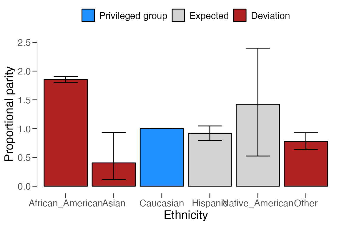

Predictive rate parity (Equalized odds): Compares the overall positive prediction rates (e.g., the precision) of each unprivileged group to the privileged group.

The formula for the precision is $PR = \frac{TP}{TP + FP}$ , and the predictive rate parity for unprivileged group $i$ is given by $PRP = \frac{PR_{i}}{PR_{privileged}}$ .
```
model_fairness(
  data = compas,
  protected = "Ethnicity",
  target = "TwoYrRecidivism",
  predictions = "Predicted",
  privileged = "Caucasian",
  positive = "yes",
  metric = "prp"
)
```
```
## 
##  Classical Algorithmic Fairness Test
## 
## data: compas
## n = 6172, X-squared = 18.799, df = 5, p-value = 0.002095
## alternative hypothesis: fairness metrics are not equal across groups
## 
## sample estimates:
##   African_American: 1.1522 [1.1143, 1.1891], p-value = 5.4523e-05
##   Asian: 0.86598 [0.11706, 1.6149], p-value = 1
##   Hispanic: 1.0229 [0.87836, 1.1611], p-value = 0.78393
##   Native_American: 1.0392 [0.25396, 1.6406], p-value = 1
##   Other: 1.0596 [0.86578, 1.2394], p-value = 0.5621
## alternative hypothesis: true odds ratio is not equal to 1
```
Interpretation:
- African American: The predictive rate parity for African Americans is 1.1522. This suggests that the precision for African Americans is approximately 1.15 times higher than for Caucasians, which indicates potential ‘favoritism’ towards African Americans in the overall positive predictions made by the algorithm.
- Asian: The predictive rate parity for Asians is 0.86598, indicating that their precision is lower than for Caucasians. This suggests potential underestimation of reoffenders among Asians by the algorithm.
- Hispanic: The predictive rate parity for Hispanics is 1.0229, suggesting their overall positive prediction rate is very close to that of the privileged group (Caucasians). This indicates relatively fair treatment in the algorithm’s overall positive predictions.
Accuracy parity: Compares the accuracy of each unprivileged group’s predictions with the privileged group.

The formula for the accuracy is $A = \frac{TP + TN}{TP + FP + TN + FN}$ , and the accuracy parity for unprivileged group $i$ is given by $AP = \frac{A_{i}}{A_{privileged}}$ .
```
model_fairness(
  data = compas,
  protected = "Ethnicity",
  target = "TwoYrRecidivism",
  predictions = "Predicted",
  privileged = "Caucasian",
  positive = "yes",
  metric = "ap"
)
```
```
## 
##  Classical Algorithmic Fairness Test
## 
## data: compas
## n = 6172, X-squared = 3.3081, df = 5, p-value = 0.6526
## alternative hypothesis: fairness metrics are not equal across groups
## 
## sample estimates:
##   African_American: 1.021 [0.99578, 1.0458], p-value = 0.29669
##   Asian: 1.1266 [0.841, 1.3384], p-value = 0.44521
##   Hispanic: 1.0351 [0.97074, 1.0963], p-value = 0.34691
##   Native_American: 0.96626 [0.46753, 1.3525], p-value = 1
##   Other: 1.0536 [0.975, 1.127], p-value = 0.21778
## alternative hypothesis: true odds ratio is not equal to 1
```
Interpretation:
- African American: The accuracy parity for African Americans is 1.021, suggesting their accuracy is very similar to the privileged group (Caucasians). This indicates fair treatment concerning overall accuracy.
- Asian: The accuracy parity for Asians is 1.1266, suggesting their accuracy is slightly higher than for Caucasians, indicating potential favoritism in overall accuracy.
- Hispanic: The accuraty parity for Hispanics is 1.0351, suggesting their accuracy is slightly higher than for Caucasians, indicating potential favoritism in overall accuracy.
False negative rate parity (Treatment equality): Compares the false negative rates of each unprivileged group with the privileged group.

The formula for the false negative rate is $FNR = \frac{FN}{TP + FN}$ , and the false negative rate parity for unprivileged group $i$ is given by $FNRP = \frac{FNR_{i}}{FNR_{privileged}}$ .
```
model_fairness(
  data = compas,
  protected = "Ethnicity",
  target = "TwoYrRecidivism",
  predictions = "Predicted",
  privileged = "Caucasian",
  positive = "yes",
  metric = "fnrp"
)
```
```
## 
##  Classical Algorithmic Fairness Test
## 
## data: compas
## n = 6172, X-squared = 246.59, df = 5, p-value < 2.2e-16
## alternative hypothesis: fairness metrics are not equal across groups
## 
## sample estimates:
##   African_American: 0.46866 [0.42965, 0.50936], p-value = < 2.22e-16
##   Asian: 1.4205 [0.66128, 1.8337], p-value = 0.29386
##   Hispanic: 1.0121 [0.87234, 1.1499], p-value = 0.93562
##   Native_American: 0.7576 [0.099899, 1.6163], p-value = 0.67157
##   Other: 1.0997 [0.92563, 1.2664], p-value = 0.28911
## alternative hypothesis: true odds ratio is not equal to 1
```
Interpretation:
- African American: The parity of false negative rates (FNRs) for African Americans compared to Caucasians is 0.46866. A value lower than 1 suggests that African Americans are less likely to be falsely classified as non-reoffenders, indicating potential bias against this group in this aspect.
- Asian: The parity for Asians is 1.4205, indicating that they are more likely to be falsely classified as non-reoffenders compared to Caucasians, suggesting potential underestimation of reoffenders among Asians.
- Hispanic: The FNR parity for Hispanics is 1.0121, indicating relatively similar rates as the privileged group (Caucasians), suggesting fair treatment in this aspect.
False positive rate parity: Compares the false positive rates (e.g., for non-reoffenders) of each unprivileged group with the privileged group.

The formula for the false positive rate is $FPR = \frac{FP}{TN + FP}$ , and the false positive rate parity for unprivileged group $i$ is given by $FPRP = \frac{FPR_{i}}{FPR_{privileged}}$ .
```
model_fairness(
  data = compas,
  protected = "Ethnicity",
  target = "TwoYrRecidivism",
  predictions = "Predicted",
  privileged = "Caucasian",
  positive = "yes",
  metric = "fprp"
)
```
```
## 
##  Classical Algorithmic Fairness Test
## 
## data: compas
## n = 6172, X-squared = 179.76, df = 5, p-value < 2.2e-16
## alternative hypothesis: fairness metrics are not equal across groups
## 
## sample estimates:
##   African_American: 1.8739 [1.7613, 1.988], p-value = < 2.22e-16
##   Asian: 0.39222 [0.048308, 1.2647], p-value = 0.19944
##   Hispanic: 0.85983 [0.67237, 1.0736], p-value = 0.25424
##   Native_American: 1.5035 [0.19518, 3.5057], p-value = 0.61986
##   Other: 0.67967 [0.47835, 0.92493], p-value = 0.019574
## alternative hypothesis: true odds ratio is not equal to 1
```
Interpretation:
- African American: The false positive rate parity for African Americans is 1.8739. This indicates that African Americans are approximately 1.87 times more likely to be falsely predicted as reoffenders than Caucasians. This suggests potential bias in the algorithm’s false positive predictions in favor of African Americans.
- Asian: The parity for Asians is 0.39222, indicating that they are less likely to be falsely predicted as reoffenders compared to Caucasians. This suggests potential fair treatment of Asians in false positive predictions.
- Hispanic: The false positive rate parity for Hispanics is 0.85983, suggesting they are less likely to be falsely predicted as reoffenders compared to Caucasians. This indicates potential fair treatment of Hispanics in false positive predictions.
True positive rate parity (Equal opportunity): Compares the true positive rates (e.g., for reoffenders) of each unprivileged group with the privileged group.

The formula for the true positive rate is $TPR = \frac{TP}{TP + FN}$ , and the true positive rate parity for unprivileged group $i$ is given by $TPRP = \frac{TPR_{i}}{TPR_{privileged}}$ .
```
model_fairness(
  data = compas,
  protected = "Ethnicity",
  target = "TwoYrRecidivism",
  predictions = "Predicted",
  privileged = "Caucasian",
  positive = "yes",
  metric = "tprp"
)
```
```
## 
##  Classical Algorithmic Fairness Test
## 
## data: compas
## n = 6172, X-squared = 246.59, df = 5, p-value < 2.2e-16
## alternative hypothesis: fairness metrics are not equal across groups
## 
## sample estimates:
##   African_American: 1.5943 [1.5488, 1.638], p-value = < 2.22e-16
##   Asian: 0.52964 [0.067485, 1.3789], p-value = 0.29386
##   Hispanic: 0.98642 [0.83236, 1.1428], p-value = 0.93562
##   Native_American: 1.2711 [0.31065, 2.0068], p-value = 0.67157
##   Other: 0.88843 [0.70202, 1.0832], p-value = 0.28911
## alternative hypothesis: true odds ratio is not equal to 1
```
Interpretation:
- African American: The true positive rate parity for African Americans is 1.5943. This indicates that African Americans are approximately 1.59 times more likely to be correctly predicted as reoffenders than Caucasians. This suggests potential favoritism towards African Americans in true positive predictions made by the algorithm.
- Asian: The parity for Asians is 0.52964, indicating that they are less likely to be correctly predicted as reoffenders compared to Caucasians. This suggests potential underestimation of reoffenders among Asians by the algorithm.
- Hispanic: The true positive rate parity for Hispanics is 0.98642, suggesting their true positive rate is very close to that of the privileged group (Caucasians). This indicates relatively fair treatment in the algorithm’s true positive predictions.
Negative predicted value parity: Compares the negative predicted value (e.g., for non-reoffenders) of each unprivileged group with that of the privileged group.

The formula for the negative predicted value is $NPV = \frac{TN}{TN + FN}$ , and the negative predicted value parity for unprivileged group $i$ is given by $NPVP = \frac{NPV_{i}}{NPV_{privileged}}$ .
```
model_fairness(
  data = compas,
  protected = "Ethnicity",
  target = "TwoYrRecidivism",
  predictions = "Predicted",
  privileged = "Caucasian",
  positive = "yes",
  metric = "npvp"
)
```
```
## 
##  Classical Algorithmic Fairness Test
## 
## data: compas
## n = 6172, X-squared = 3.6309, df = 5, p-value = 0.6037
## alternative hypothesis: fairness metrics are not equal across groups
## 
## sample estimates:
##   African_American: 0.98013 [0.94264, 1.0164], p-value = 0.45551
##   Asian: 1.1163 [0.82877, 1.3116], p-value = 0.52546
##   Hispanic: 1.0326 [0.96161, 1.0984], p-value = 0.43956
##   Native_American: 0.95687 [0.31975, 1.3732], p-value = 1
##   Other: 1.0348 [0.95007, 1.112], p-value = 0.46084
## alternative hypothesis: true odds ratio is not equal to 1
```
Interpretation:
- African American: The negative predicted value parity for African Americans is 0.98013. A value close to 1 indicates that the negative predicted value for African Americans is very similar to the privileged group (Caucasians). This suggests fair treatment in predicting non-reoffenders among African Americans.
- Asian: The negative predicted value parity for Asians is 1.1163, indicating that their negative predicted value is slightly higher than for Caucasians. This could suggest potential favoritism towards Asians in predicting non-reoffenders.
- Hispanic: The negative predicted value parity for Hispanics is 1.0326, suggesting that their negative predicted value is slightly higher than for Caucasians. This indicates potential favoritism towards Hispanics in predicting non-reoffenders.
Specificity parity (True negative rate parity): Compares the specificity (true negative rate) of each unprivileged group with the privileged group.

The formula for the specificity is $S = \frac{TN}{TN + FP}$ , and the specificity parity for unprivileged group $i$ is given by $SP = \frac{S_{i}}{S_{privileged}}$ .
```
model_fairness(
  data = compas,
  protected = "Ethnicity",
  target = "TwoYrRecidivism",
  predictions = "Predicted",
  privileged = "Caucasian",
  positive = "yes",
  metric = "sp"
)
```
```
## 
##  Classical Algorithmic Fairness Test
## 
## data: compas
## n = 6172, X-squared = 179.76, df = 5, p-value < 2.2e-16
## alternative hypothesis: fairness metrics are not equal across groups
## 
## sample estimates:
##   African_American: 0.75105 [0.71855, 0.78314], p-value = < 2.22e-16
##   Asian: 1.1731 [0.92461, 1.2711], p-value = 0.19944
##   Hispanic: 1.0399 [0.97904, 1.0933], p-value = 0.25424
##   Native_American: 0.85657 [0.28624, 1.2293], p-value = 0.61986
##   Other: 1.0912 [1.0214, 1.1486], p-value = 0.019574
## alternative hypothesis: true odds ratio is not equal to 1
```
Interpretation:
- African American: The specificity parity for African Americans is 0.75105. A value lower than 1 indicates that the specificity for African Americans is lower than for Caucasians. This suggests potential bias in correctly identifying non-reoffenders among African Americans.
- Asian: The specificity parity for Asians is 1.1731, indicating their specificity is slightly higher than for Caucasians. This could suggest potential favoritism in correctly identifying non-reoffenders among Asians.
- Hispanic: The specificity parity for Hispanics is 1.0399, suggesting that their specificity is very close to the privileged group. This indicates relatively fair treatment in correctly identifying non-reoffenders among Hispanics.

Bayesian Analysis

Bayesian inference, which is supported for all metrics except demographic parity, provides credible intervals and Bayes factors for the fairness metrics and tests (Jamil et al., 2017). Similar to other functions in jfa, a Bayesian analysis can be conducted using a default prior by setting prior = TRUE. The prior distribution in this analysis is specified on the log odds ratio and can be modified by setting prior = 1 (equal to prior = TRUE), or providing a number greater than one that represents the prior concentration parameter (for example, prior = 3). The larger the concentration parameter, the more the prior distribution is focused around zero, implying that it assigns a higher probability to the scenario of equal fairness metrics.

x <- model_fairness(
  data = compas,
  protected = "Ethnicity",
  target = "TwoYrRecidivism",
  predictions = "Predicted",
  privileged = "Caucasian",
  positive = "yes",
  metric = "pp",
  prior = TRUE
)
print(x)

## 
##  Bayesian Algorithmic Fairness Test
## 
## data: compas
## n = 6172, BF₁₀ = 9.3953e+107
## alternative hypothesis: fairness metrics are not equal across groups
## 
## sample estimates:
##   African_American: 1.8505 [1.7986, 1.9066], BF₁₀ = 4.1528e+81
##   Asian: 0.32748 [0.16714, 0.93262], BF₁₀ = 0.26796
##   Hispanic: 0.92228 [0.8021, 1.0434], BF₁₀ = 0.10615
##   Native_American: 1.4864 [0.64076, 2.2547], BF₁₀ = 0.018438
##   Other: 0.73551 [0.64728, 0.92786], BF₁₀ = 1.815
## alternative hypothesis: true odds ratio is not equal to 1

The Bayes factor $BF_{01}$ , used in Bayesian inference, quantifies the evidence supporting algorithmic fairness (i.e., equal fairness metrics across all groups) over algorithmic bias. Conversely, $BF_{10}$ quantifies the evidence supporting algorithmic bias over algorithmic fairness. By default, jfa reports $BF_{10}$ , but $BF_{01}$ = $\frac{1}{BF_{10}}$ . The output above shows the resulting Bayes factor ( $BF_{01}$ ) in favor of rejecting the null hypothesis of algorithmic fairness. As shown, $BF_{01}$ > 1000, indicating extreme evidence against the hypothesis of equal fairness metrics between the groups.

The prior and posterior distribution for the group comparisons can be visualized by invoking plot(..., type = "posterior").

plot(x, type = "posterior")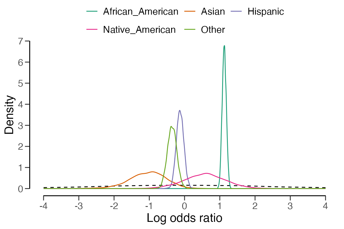

Additionally, the robustness of the Bayes factor to the choice of prior distribution can be examined by calling plot(..., type = "robustness"), as shown in the code below. Finally, the auditor has the option to conduct a sequential analysis using plot(..., type = "sequential").

plot(x, type = "robustness")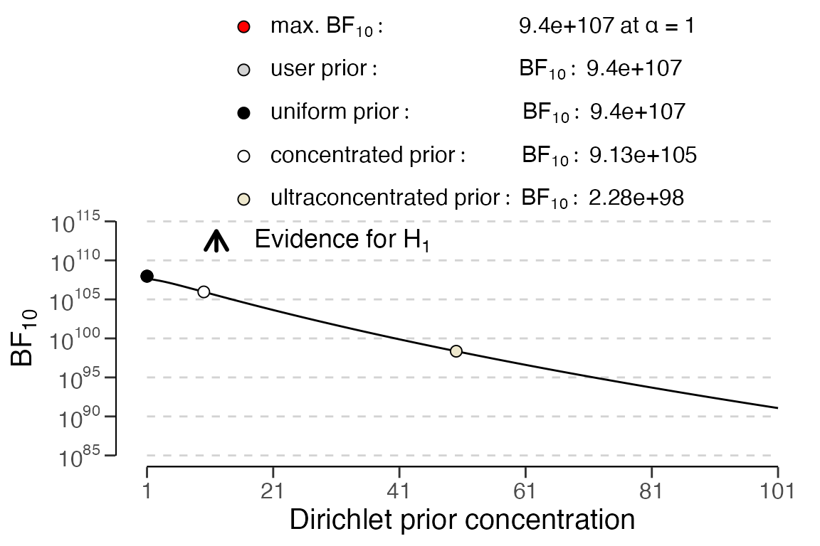

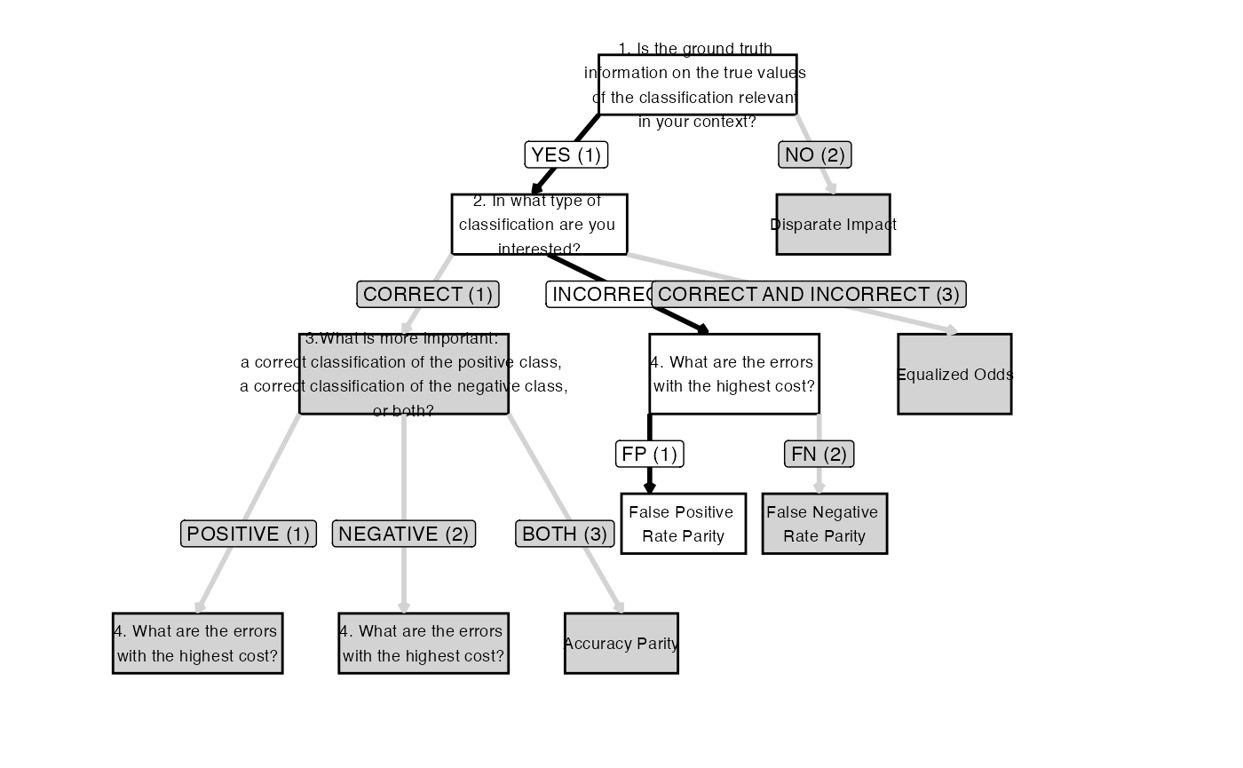
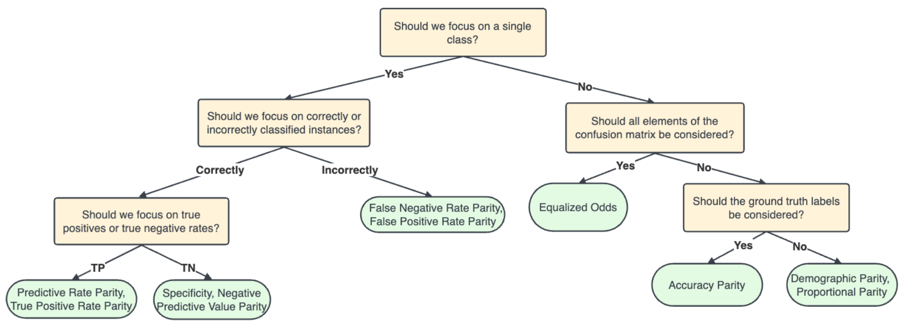
Function: `fairness_selection()`

The fairness_selection() function offers a method to select a fairness measure tailored to a specific context and dataset by answering the questions in the developed decision-making workflow. The fairness measure that can be selected include disparate impact, equalized odds, false positive rate parity, false negative rate parity, predictive rate parity, equal opportunity, specificity parity, negative predictive value parity, accuracy parity Verma & Rubin (2018). After answering the questions in the decision-making workflow and selecting the fairness measure to apply, a graphical representation of the followed path can be created based on the responses.

As mentioned earlier, not all fairness measures are equally suitable for every audit situation. For this reason, the fairness_selection() function we propose can assist the auditor in selecting the most appropriate measure for the specific audit at hand. To demonstrate the usage of the fairness_selection() function, we will answer each necessary question in the decision-making workflow, explaining the reasoning behind each response.

The first question in the workflow checks if the dataset includes the ground truth information (i.e., the true classification values). The data available in this dataset were collected during a retrospective study, so we have information on whether offenders committed a crime within 2 years of being released (TwoYrRecidivism). Therefore, we can answer the first question with Yes (in the function the value 1 is used to indicate Yes).

The second question focuses on the type of classification of interest: correct, incorrect, or both. We can imagine a scenario where the analysis of this dataset is tied to U.S. Attorney General Eric Holder’s concerns about potential discrimination against certain social groups resulting from anomalies in AI-generated classifications, particularly errors in classifying offenders. Given the importance of identifying such irregularities, our focus here is on the incorrect classification of offenders. Therefore, we can answer the first question with Incorrect Classification (in the function the value 2 is used to indicate Incorrect Classification).

Given the answer to the second question and following the decision-making workflow path, we can skip the third question and proceed directly to the fourth and final question.

The fourth question addresses the costs of classification errors meaning which classification error results in highest cost. The classification errors can be made when classifying someone who would not commit another crime within two years of release as someone who would (leading a longer incarceration or failing to release someone from prison in a timely manner) and when classifying a dangerous individual who would commit another crime as someone who would not (leading to an early release or shorter incarceration period). To answer the question, we assume a scenario where AI is being developed and promoted within the U.S. criminal justice system, with the goal of reducing incarceration and alleviating prison overcrowding. Thus, higher costs are associated with mistakenly incarcerating individuals who would not reoffend within two years of release, as this results in unnecessary prolonged imprisonment. Therefore, we can answer the fourth question with False Positive (in the function the value 1 is used to indicate False Positive).

measure <- fairness_selection(q1 = 1, q2 = 2, q4 = 1)
print(measure)

## 
##  Fairness Measure for Model Evaluation
## 
## Selected fairness measure: False Positive Rate Parity 
## 
## Based on:
##   Answer to question 1 (q1): Yes (1)
##   Answer to question 2 (q2): Incorrect classification (2)
##   Answer to question 4 (q4): False Positive (1)

It is worth noting that the function can also be called without any arguments (measure <- fairness_selection()). In this case, an interactive mode is activated, allowing the user to answer the necessary questions in real time. By applying this function, an object of class jfaFairnessSelection is created.

Additionally, the print function, applied to an object of class jfaFairnessSelection, allows us to display not only which fairness measure is selected as the most suitable for the audit situation, but also a summary of how we answered the questions in the decision-making workflow.

Finally, as mentioned earlier, it is possible to visualize the path followed by answering the questions in the decision-making workflow. This is done by applying the plot function an object of class jfaFairnessSelection.

plot(measure)

References

Calders, T., & Verwer, S. (2010). Three naive Bayes approaches for discrimination-free classification. Data Mining and Knowledge Discovery. https://doi.org/10.1007/s10618-010-0190-x

Castelnovo, A., Crupi, R., Greco, G., Regoli, D., Penco, I. G., & Cosentini, A. C. (2022). A clarification of the nuances in the fairness metrics landscape. Scientific Reports, 12(1), 4209. https://doi.org/10.1038/s41598-022-07939-1

Chouldechova, A. (2017). Fair prediction with disparate impact: A study of bias in recidivism prediction instruments. Big Data. https://doi.org/10.1089/big.2016.0047

Feldman, M., Friedler, S. A., Moeller, J., Scheidegger, C., & Venkatasubramanian, S. (2015). Certifying and removing disparate impact. Proceedings of the 21th ACM SIGKDD International Conference on Knowledge Discovery and Data Mining. https://doi.org/10.1145/2783258.2783311

Fisher, R. A. (1970). Statistical methods for research workers. Oliver & Boyd.

Friedler, S. A., Scheidegger, C., Venkatasubramanian, S., Choudhary, S., Hamilton, E. P., & Roth, D. (2019). A comparative study of fairness-enhancing interventions in machine learning. Proceedings of the Conference on Fairness, Accountability, and Transparency. https://doi.org/10.1145/3287560.3287589

Hardt, M., Price, E., & Srebro, N. (2016). Equality of opportunity in supervised learning. Advances in Neural Information Processing Systems, 29. https://doi.org/10.48550/arXiv.1610.02413

Jamil, T., Ly, A., Morey, R. D., Love, J., Marsman, M., & Wagenmakers, E.-J. (2017). Default "Gunel and Dickey" Bayes factors for contingency tables. Behavior Research Methods, 49, 638–652. https://doi.org/10.3758/s13428-016-0739-8

Pessach, D., & Shmueli, E. (2022). A review on fairness in machine learning. ACM Computing Surveys, 55(3), 1–44. https://doi.org/10.1145/3494672

Verma, S., & Rubin, J. (2018). Fairness definitions explained. Proceedings of the International Workshop on Software Fairness, 1–7. https://doi.org/10.1145/3194770.3194776

Zafar, M. B., Valera, I., Gomez Rodriguez, M., & Gummadi, K. P. (2017). Fairness beyond disparate treatment & disparate impact. Proceedings of the 26th International Conference on World Wide Web. https://doi.org/10.1145/3038912.3052660

Koen Derks

Introduction

Function: model_fairness()

Bayesian Analysis

Function: fairness_selection()

References

Function: `model_fairness()`

Function: `fairness_selection()`