data(BuildIt)
n <- 105 Selection
Auditors must often evaluate balances or populations that include a large quantity of items. As it is not possible to individually examine all of these items, they must select a subset, or sample, from the total population to make a statement about a specific characteristic of the population. Several selection methodologies, which are widely accepted in the audit context, are available for this purpose. This chapter discusses the most frequently used sampling methodology for audit sampling and demonstrates how to select a sample using these methods in R.
5.1 Sampling Units
Selecting a subset from the population requires knowledge of the sampling units; physical representations of the population that needs to be audited. Generally, the auditor has to choose between two types of sampling units: individual items in the population or individual monetary units in the population. In order to perform statistical selection, the population must be divided into individual sampling units that can be assigned a probability to be included in the sample. The total collection of all sampling units which have been assigned a selection probability is called the sampling frame.
5.1.1 Items
A sampling unit for record (i.e., attributes) sampling is generally a characteristic of an item in the population. For example, suppose that you inspect a population of receipts. A possible sampling unit for record sampling can be the date of payment of the receipt. When a sampling unit (e.g., date of payment) is selected by the sampling method, the population item that corresponds to the sampled unit is included in the sample.
5.1.2 Monetary Units
A sampling unit for monetary unit sampling is different than a sampling unit for record sampling in that it is an individual monetary unit within an item or transaction, like an individual dollar. For example, a single sampling unit can be the 10\(^{\text{th}}\) dollar from a specific receipt in the population. When a sampling unit (e.g., individual dollar) is selected by the sampling method, the population item that includes the sampling unit is included in the sample.
5.2 Sampling Methods
This section discusses four sampling methods that are commonly used in audit sampling. The methods that will be discussed are:
- Random sampling
- Fixed interval sampling
- Cell sampling
- Modified sieve sampling
First, let’s get some notation out of the way. As discussed in Chapter 2, the population size \(N\) is defined as the total set of individual sampling units (denoted by \(x_i\)).
\[\begin{equation} N = \{x_1, x_2, \dots, x_N\}. \end{equation}\]
In statistical sampling, every sampling unit \(x_i\) in the population should receive a selection probability \(p(x_i)\). The purpose of the sampling method is to provide a framework to assign selection probabilities to each of the sampling units, and subsequently draw sampling units from the population until a set of size \(n\) has been created.
To illustrate how the resulting sample differs for various sampling methods, we will use the BuildIt data set included in the jfa package. These data can be loaded into R using the code below. For simplicity, we will use a sample size of \(n\) = 10 for all examples.
5.2.1 Random Sampling
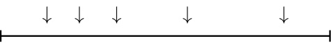
Random sampling is the most simple and straight-forward selection method. The random sampling method provides a method that allows every sampling unit in the population an equal chance of being selected, meaning that every combination of sampling units has the same probability of being selected as every other combination of the same number of sampling units. Simply put, the algorithm draws a random selection of size \(n\) of the sampling units. Therefore, the selection probability for each sampling unit is defined as:
\[\begin{equation} p(x) = \frac{1}{N}. \end{equation}\]
To make this procedure visually intuitive, Figure 5.1 below provides an illustration of the random sampling method.
- Advantage(s): The random sampling method yields an optimal random selection, with the additional advantage that the sample can be easily extended by applying the same method again.
- Disadvantages: Because the selection probabilities are equal for all sampling units there is no guarantee that items with a large monetary value in the population will be included in the sample.
5.2.1.1 Record Sampling
Random sampling can easily be coded in base R. First, we have to get a vector of of the possible items (rows) in the population that can be selected. When we are performing record sampling, we can simply use R’s build in sample() function to draw a random sample from a vector 1:nrow(BuildIt) representing the row indices of the items and store the result in a variable items.
set.seed(1)
items <- sample.int(nrow(BuildIt), size = n, replace = FALSE)
items
#>  [1] 1017  679 2177  930 1533  471 2347  270 1211 3379
You can then select the sample from the population using the selected indices stored in items.
BuildIt[items, ]
#>         ID bookValue auditValue
#> 1017 50755    618.24     618.24
#> 679  20237    669.75     669.75
#> 2177  9517    454.02     454.02
#> 930  85674    257.82     257.82
#> 1533 31051    308.53     308.53
#> 471  84375    824.66     824.66
#> 2347 75616    623.70     623.70
#> 270  82033    352.75     352.75
#> 1211 12877     52.89      52.89
#> 3379 85322    330.24     330.24
The sample can be reproduced in jfa via the selection() function. This function takes as input the population data, the sample size, and the characteristics of the sampling method. The argument units allows you to specify that you want to use record sampling (units = "items"), while the method argument enables you to specify that you are performing random sampling (method = 'random').
set.seed(1)
selection(BuildIt, size = n, units = "items", method = "random")$sample
#>     row times    ID bookValue auditValue
#> 1  1017     1 50755    618.24     618.24
#> 2   679     1 20237    669.75     669.75
#> 3  2177     1  9517    454.02     454.02
#> 4   930     1 85674    257.82     257.82
#> 5  1533     1 31051    308.53     308.53
#> 6   471     1 84375    824.66     824.66
#> 7  2347     1 75616    623.70     623.70
#> 8   270     1 82033    352.75     352.75
#> 9  1211     1 12877     52.89      52.89
#> 10 3379     1 85322    330.24     330.24
An alternative to specifying the desired sample size through the size argument is to provide an object generated by the planning() function to the selection() function. For instance, the following code utilizes the planning() function to plan a sample size based on a performance materiality of 0.03, or three percent, and a sampling risk of 0.05, or five percent, which can be passed directly to selection() to select the sample from the BuildIt population.
selection(BuildIt, size = planning(materiality = 0.03), units = "items", method = "random")
#>
#>  Audit Sample Selection
#>
#> data:  BuildIt
#> number of sampling units = 100, number of items = 100
#> sample selected via method 'items' + 'random'
The ability of one function to accept input from another function allows for the implementation of a workflow in which the planning() function and the selection() function are sequentially linked. Additionally, the use of R’s native pipe operator |> further simplifies this process.
planning(materiality = 0.03) |>
  selection(data = BuildIt, units = "items", method = "random")
#>
#>  Audit Sample Selection
#>
#> data:  BuildIt
#> number of sampling units = 100, number of items = 100
#> sample selected via method 'items' + 'random'
The selection() function has three additional arguments which you can use to preprocess your population before selection. These arguments are order, decreasing and randomize.
The order argument takes as input a column name in data which determines the order of the population. For example, you can order the population from lowest book value to highest book value before engaging in the selection. In this case, you should use the decreasing = FALSE (its default value) argument.
set.seed(1)
selection(BuildIt, size = n, order = "bookValue", units = "items", method = "random")$sample
#>     row times    ID bookValue auditValue
#> 1    29     1 58849    274.26     274.26
#> 2  3297     1 24279    229.95     229.95
#> 3   931     1 28025    429.14     429.14
#> 4   756     1 11563    263.08     105.23
#> 5  3375     1 58981    335.39     335.39
#> 6  1624     1 97783    197.19     197.19
#> 7  2534     1 95715    457.42     457.42
#> 8  1798     1 95520    157.54     157.54
#> 9  3448     1 12959    296.82     296.82
#> 10  450     1 39908    831.31     831.31
The randomize argument can be used to randomly shuffle the items in the population before selection. For example, you can randomly shuffle the population before engaging in the selection using randomize = TRUE.
set.seed(1)
selection(BuildIt, size = n, randomize = TRUE, units = "items", method = "random")$sample
#>     row times    ID bookValue auditValue
#> 1  1264     1 85424    406.81     406.81
#> 2   923     1 12566    287.61     287.61
#> 3   776     1 92923    247.89     247.89
#> 4   127     1 71325    306.78     306.78
#> 5  1611     1 10019    191.18     191.18
#> 6  3087     1 87887    666.13     666.13
#> 7  1729     1 78779    608.02     608.02
#> 8  2037     1 74155    347.18     347.18
#> 9  2769     1 26010    240.10     240.10
#> 10 2276     1 80154    282.91     282.91
5.2.1.2 Monetary Unit Sampling
When we are performing record sampling, we have to consider that each item in the population consists of multiple smaller items (i.e., the monetary units), which means that items with a higher book value should get a higher probability of being selected. The sample() function faciliates weighted selection via the prob argument, which takes a vector of values and, using normalization, computes the weights for selection. The call below is similar to before, but in this case we use the book values in the column bookValues of the data set to weigh the items and store the result in a variable items.
set.seed(1)
items <- sample.int(nrow(BuildIt), size = n, replace = TRUE, prob = BuildIt[["bookValue"]])
items
#>  [1] 1017  679 2856  471  270 2642  597 2208  330 1615
You can then select the sample from the population using the selected indices stored in items.
BuildIt[items, ]
#>         ID bookValue auditValue
#> 1017 50755    618.24     618.24
#> 679  20237    669.75     669.75
#> 2856 21836    820.86     820.86
#> 471  84375    824.66     824.66
#> 270  82033    352.75     352.75
#> 2642 49666    601.71     601.71
#> 597  93226    376.55     376.55
#> 2208 61540    963.53     963.53
#> 330  30774    508.26     508.26
#> 1615 42859    598.07     598.07
The sample can be reproduced in jfa via the selection() function. The argument units allows you to specify that you want to use monetary unit sampling (units = "values"), while the method argument enables you to specify that you are performing random sampling (method = 'random'). Note that you should provide the name of the column in the data that contains the monetary units via the values argument.
set.seed(1)
selection(BuildIt, size = n, units = "values", method = "random", values = "bookValue")$sample
#>     row times    ID bookValue auditValue
#> 1  1017     1 50755    618.24     618.24
#> 2   679     1 20237    669.75     669.75
#> 3  2856     1 21836    820.86     820.86
#> 4   471     1 84375    824.66     824.66
#> 5   270     1 82033    352.75     352.75
#> 6  2642     1 49666    601.71     601.71
#> 7   597     1 93226    376.55     376.55
#> 8  2208     1 61540    963.53     963.53
#> 9   330     1 30774    508.26     508.26
#> 10 1615     1 42859    598.07     598.07
5.2.2 Fixed Interval Sampling
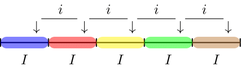
Fixed interval sampling is a method designed for yielding representative samples from monetary populations. The algorithm determines a uniform interval on the (optionally ranked) sampling units. Next, a starting point is handpicked or randomly selected in the first interval and a sampling unit is selected throughout the population at each of the uniform intervals from the starting point. For example, if the interval has a width of 10 sampling units and sampling unit number 5 is chosen as the starting point, the sampling units 5, 15, 25, etc. are selected to be included in the sample.
The number of required intervals \(I\) can be determined by dividing the number of sampling units in the population by the required sample size:
\[\begin{equation} I = \frac{N}{n}, \end{equation}\]
in which \(n\) is the required sample size and \(N\) is the total number of sampling units in the population.
If the space between the selected sampling units is equal, the selection probability for each sampling unit is theoretically defined as:
\[\begin{equation} p(x) = \frac{1}{I}, \end{equation}\]
with the property that the space between selected units \(i\) (of which the first one is the starting point) is the same as the interval \(I\), see @#fig-selection-interval below. However, in practice the selection is deterministic and completely depends on the chosen starting points (using start).
The fixed interval method yields a sample that allows every sampling unit in the population an equal chance of being selected. However, the fixed interval method has the property that all items in the population with a monetary value larger than the interval \(I\) have an selection probability of one because one of these items’ sampling units are always selected from the interval. Note that, if the population is arranged randomly with respect to its deviation pattern, fixed interval sampling is equivalent to random selection.
- Advantage(s): The advantage of the fixed interval sampling method is that it is often simple to understand and fast to perform. Another advantage is that, in monetary unit sampling, all items that are greater than the calculated interval will be included in the sample. In record sampling, since units can be ranked on the basis of value, there is also a guarantee that some large items will be in the sample.
- Disadvantage(s): A pattern in the population can coincide with the selected interval, rendering the sample less representative. What is sometimes seen as an added complication for this method is that the sample is hard to extend after drawing the initial sample. This is due to the chance of selecting the same sampling unit. However, by removing the already selected sampling units from the population and redrawing the intervals this problem can be efficiently solved.
5.2.2.1 Record Sampling
To code fixed interval sampling in a record sampling context, we first have to compute the size of the interval we are working with. This is computed by dividing the number of items in the population by the desired sample size \(n\). Suppose the auditor wants to select a sample of 10 items, then the interval is computed by:
interval <- nrow(BuildIt) / nNext, we have to determine the starting point. We are going to take the fifth unit in each interval in this case.
start <- 5To find which rows are part of the sample, we execute the following code:
items <- ceiling(start + interval * 0:(n - 1))You can then select the sample from the population using the selected indices stored in items.
BuildIt[items, ]
#>         ID bookValue auditValue
#> 5    55080    620.88     620.88
#> 355  27934    749.38     749.38
#> 705  21900    919.00     919.00
#> 1055 66675    384.27     384.27
#> 1405 13472    360.05     360.05
#> 1755 61607    389.75     389.75
#> 2105 68519    354.71     354.71
#> 2455 91983    467.72     467.72
#> 2805 25646    420.80     420.80
#> 3155 94955    248.77     248.77
The sample can be reproduced in jfa via the selection() function. The argument units allows you to specify that you want to use record sampling (units = "items"), while the method argument enables you to specify that you are performing fixed interval sampling (method = 'interval'). Note that, by default, the first sampling unit from each interval is selected. However, this can be changed by setting the argument start to a different value.
selection(BuildIt, size = n, units = "items", method = "interval", start = start)$sample
#>     row times    ID bookValue auditValue
#> 1     5     1 55080    620.88     620.88
#> 2   355     1 27934    749.38     749.38
#> 3   705     1 21900    919.00     919.00
#> 4  1055     1 66675    384.27     384.27
#> 5  1405     1 13472    360.05     360.05
#> 6  1755     1 61607    389.75     389.75
#> 7  2105     1 68519    354.71     354.71
#> 8  2455     1 91983    467.72     467.72
#> 9  2805     1 25646    420.80     420.80
#> 10 3155     1 94955    248.77     248.77
5.2.2.2 Monetary Unit Sampling
In monetary unit sampling, the only difference is that we are computing the interval on the basis of the booked values in the column bookValue of the data set. In this case, the starting point start = 5 determines which monetary unit from each interval is selected.
interval <- sum(BuildIt[["bookValue"]]) / nTo find which units are part of the sample, we execute the following code:
units <- start + interval * 0:(n - 1)To obtain which items are part of the sample, we can run the following for loop. Note that this does not take into account whether the book values contain negative values, which should not be included in the cumulative sum below.
You can then select the sample from the population using the selected indices stored in items.
BuildIt[items, ]
#>         ID bookValue auditValue
#> 1    82884    242.61     242.61
#> 358  20711    610.88     610.88
#> 715  99012    313.75     313.75
#> 1081 65319    502.54     201.02
#> 1421 88454    856.28     856.28
#> 1774 87258    157.68     157.68
#> 2103 48652    497.21     497.21
#> 2435 37248   1041.44    1041.44
#> 2787 10925    377.10     377.10
#> 3152 71832   1001.82    1001.82
The sample can be reproduced in jfa via the selection() function. The argument units allows you to specify that you want to use monetary unit sampling (units = "values"), while the method argument enables you to specify that you are performing fixed interval sampling (method = 'interval'). Note that you should provide the name of the column in the data that contains the monetary units via the values argument.
selection(BuildIt, size = n, units = "values", method = "interval", values = "bookValue", start = start)$sample
#>     row times    ID bookValue auditValue
#> 1     1     1 82884    242.61     242.61
#> 2   358     1 20711    610.88     610.88
#> 3   715     1 99012    313.75     313.75
#> 4  1081     1 65319    502.54     201.02
#> 5  1421     1 88454    856.28     856.28
#> 6  1774     1 87258    157.68     157.68
#> 7  2103     1 48652    497.21     497.21
#> 8  2435     1 37248   1041.44    1041.44
#> 9  2787     1 10925    377.10     377.10
#> 10 3152     1 71832   1001.82    1001.82
5.2.3 Cell Sampling
The cell sampling method divides the (optionally ranked) population into a set of intervals \(I\) that are computed through the previously given equations. Within each interval, a sampling unit is selected by randomly drawing a number between 1 and the interval range \(I\). This causes the space \(i\) between the sampling units to vary. The procedure is displayed in @#fig-selection-cell.
Like in the fixed interval sampling method, the selection probability for each sampling unit is defined as:
\[\begin{equation} p(x) = \frac{1}{I}. \end{equation}\]
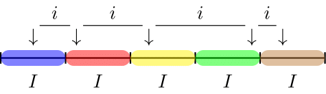
The cell sampling method has the property that all items in the population with a monetary value larger than twice the interval \(I\) have a selection probability of one.
- Advantage(s): More sets of samples are possible than in fixed interval sampling, as there is no systematic interval \(i\) to determine the selections. It is argued that the cell sampling algorithm offers a solution to the pattern problem in fixed interval sampling.
- Disadvantage(s): A disadvantage of this sampling method is that not all items in the population with a monetary value larger than the interval have a selection probability of one. Besides, population items can be in two adjacent cells, thereby creating the possibility that an items is included in the sample twice.
5.2.3.1 Record Sampling
To code cell sampling in a record sampling context, we again have to compute the size of the interval we are working with:
interval <- nrow(BuildIt) / nNext, we have to randomly determine which items are going to be selected in each interval.
To find which rows are part of the sample, we execute the following code:
items <- floor(starts + interval * 0:(n - 1))You can then select the sample from the population using the selected indices stored in items.
BuildIt[items, ]
#>         ID bookValue auditValue
#> 92   75133    355.16     355.16
#> 480  81037    456.27     456.27
#> 900   1730    449.87     449.87
#> 1367 36587    282.32     282.32
#> 1470 10305    648.70     648.70
#> 2064 96344    268.94     268.94
#> 2430 60885    493.77     493.77
#> 2681 60935    312.98     312.98
#> 3020  8716    450.76     450.76
#> 3171 61036    387.67     387.67
The sample can be reproduced in jfa via the selection() function. The argument units allows you to specify that you want to use record sampling (units = "items"), while the method argument enables you to specify that you are performing cell sampling (method = 'cell').
set.seed(1)
selection(BuildIt, size = n, units = "items", method = "cell")$sample
#>     row times    ID bookValue auditValue
#> 1    92     1 75133    355.16     355.16
#> 2   480     1 81037    456.27     456.27
#> 3   900     1  1730    449.87     449.87
#> 4  1367     1 36587    282.32     282.32
#> 5  1470     1 10305    648.70     648.70
#> 6  2064     1 96344    268.94     268.94
#> 7  2430     1 60885    493.77     493.77
#> 8  2681     1 60935    312.98     312.98
#> 9  3020     1  8716    450.76     450.76
#> 10 3171     1 61036    387.67     387.67
5.2.3.2 Monetary Unit Sampling
In monetary unit sampling, the only difference is that we are computing the interval on the basis of the booked values in the column bookValue of the data set. In this case, the starting points start determines which monetary unit from each interval is selected.
interval <- sum(BuildIt[["bookValue"]]) / nTo obtain which items are part of the sample, we can run the following for loop. Note that this does not take into account whether the book values contain negative values, which should not be included in the cumulative sum below.
set.seed(1)
all_units <- ifelse(BuildIt[["bookValue"]] < 0, 0, BuildIt[["bookValue"]])
all_items <- 1:nrow(BuildIt)
intervals <- 0:n * interval
items <- numeric(n)
for (i in 1:n) {
  unit <- stats::runif(1, intervals[i], intervals[i + 1])
  item <- which(unit <= cumsum(all_units))[1]
  items[i] <- all_items[item]
}
You can then select the sample from the population using the selected indices stored in items.
BuildIt[items, ]
#>         ID bookValue auditValue
#> 95   15009    415.60     415.60
#> 486  79093    635.85     635.85
#> 931  28025    429.14     429.14
#> 1387 56444    296.37     296.37
#> 1492 81443    543.80     543.80
#> 2074 14196    270.45     270.45
#> 2418 87743    347.99     347.99
#> 2660 23927    454.81     454.81
#> 3024 78925    251.44     251.44
#> 3172 18286    450.57     450.57
The sample can be reproduced in jfa via the selection() function. The argument units allows you to specify that you want to use monetary unit sampling (units = "values"), while the method argument enables you to specify that you are performing cell sampling (method = 'cell'). Note that you should provide the name of the column in the data that contains the monetary units via the values argument.
set.seed(1)
selection(BuildIt, size = n, units = "values", method = "cell", values = "bookValue")$sample
#>     row times    ID bookValue auditValue
#> 1    95     1 15009    415.60     415.60
#> 2   486     1 79093    635.85     635.85
#> 3   931     1 28025    429.14     429.14
#> 4  1387     1 56444    296.37     296.37
#> 5  1492     1 81443    543.80     543.80
#> 6  2074     1 14196    270.45     270.45
#> 7  2418     1 87743    347.99     347.99
#> 8  2660     1 23927    454.81     454.81
#> 9  3024     1 78925    251.44     251.44
#> 10 3172     1 18286    450.57     450.57
5.2.4 Modified Sieve Sampling
The fourth option for the sampling method is modified sieve sampling (Hoogduin, Hall, & Tsay, 2010). The algorithm starts by selecting a standard uniform random number \(R_i\) between 0 and 1 for each item in the population. Next, the sieve ratio:
\[\begin{equation} S_i = \frac{Y_i}{R_i} \end{equation}\]
is computed for each item by dividing the book value of that item by the random number. Lastly, the items in the population are sorted by their sieve ratio \(S\) (in decreasing order) and the top \(n\) items are selected for inspection. In contrast to the classical sieve sampling method (Rietveld, 1978), the modified sieve sampling method provides precise control over sample sizes.
5.2.4.1 Monetary Unit Sampling
You can then select the sample from the population using the selected indices stored in items.
BuildIt[items, ]
#>         ID bookValue auditValue
#> 2329 29919    681.10     681.10
#> 2883 59402    279.29     279.29
#> 1949 56012    581.22     581.22
#> 3065 47482    621.73     621.73
#> 1072 79901    789.97     789.97
#> 488  50811    651.35     651.35
#> 1916 53565    266.37     266.37
#> 463  65768    480.89     480.89
#> 1311 91955    398.96     398.96
#> 2895  8688    492.02     492.02
The sample can be reproduced in jfa via the selection() function. The argument units allows you to specify that you want to use monetary unit sampling (units = "values"), while the method argument enables you to specify that you are performing modified sieve sampling (method = 'sieve'). Note that you should provide the name of the column in the data that contains the monetary units via the values argument.
set.seed(1)
selection(BuildIt, size = n, units = "values", method = "sieve", values = "bookValue")$sample
#>     row times    ID bookValue auditValue
#> 1  2329     1 29919    681.10     681.10
#> 2  2883     1 59402    279.29     279.29
#> 3  1949     1 56012    581.22     581.22
#> 4  3065     1 47482    621.73     621.73
#> 5  1072     1 79901    789.97     789.97
#> 6   488     1 50811    651.35     651.35
#> 7  1916     1 53565    266.37     266.37
#> 8   463     1 65768    480.89     480.89
#> 9  1311     1 91955    398.96     398.96
#> 10 2895     1  8688    492.02     492.02
5.3 Practical Exercises
- Select a random sample of 120 items from the
BuildItdata set.
Click to reveal answer
Selecting a random sample of items can be done using the selection() function with the additional arguments size = 120, method = "random" and units = "items".
selec <- selection(data = BuildIt, size = 120, method = "random", units = "items")
head(selec[["sample"]], 5)
#>    row times    ID bookValue auditValue
#> 1 2453     1 95755    295.58     295.58
#> 2 2914     1 86541    470.99     470.99
#> 3  301     1 61726    588.81     588.81
#> 4 2632     1  3335    237.32     237.32
#> 5 1579 1 62317 309.74 309.74- Select a sample of 240 monetary units from the
BuildItdata set using a fixed interval selection method. Use a starting point of 12.
Click to reveal answer
Selecting a random sample of items can be done using the selection() function with the arguments size = 240, method = "interval" and units = "values". Additionally, for fixed interval monetary unit sampling, the book values must be given in via argument values = "bookValue". The starting point is indicated using start = 12.
selec <- selection(data = BuildIt, size = 240, method = "interval", units = "values", values = "bookValue", start = 12)
head(selec[["sample"]], 5)
#>   row times    ID bookValue auditValue
#> 1   1     1 82884    242.61     242.61
#> 2  15     1 76073    469.93     469.93
#> 3  31     1 83557    507.34     507.34
#> 4  47     1 53784    325.19     325.19
#> 5  63     1 51272    248.40     248.40