Evaluating statistical audit samples

Introduction

Welcome to the ‘Evaluating statistical audit samples’ vignette of the jfa package. This page demonstrates how to evaluate the misstatement in an audit sample using the evaluation() function in package.

evaluation

In auditing, the objective of evaluation is typically 1) to estimate the misstatement in the population based on a sample or 2) to test the misstatement against a critical upper limit, known as performance materiality.

Required information

Firstly, to evaluate an audit sample using the evaluation() function, the sample data must be available in one of two formats:

Summary statistics: This includes (a vector of) the number of items (n), (a vector of) the sum of misstatements/taints (x) and optionally (a vector of) the number of units in the population (N.units).
Data: A data.frame that contains a numeric column with book values (values), a numeric column with audit (i.e., true) values (values.audit), and optionally a factor column indicating stratum membership (strata).

By default, evaluation() estimates the population misstatement and returns a point estimate as well as a confidence/credible interval around this estimate, expressed as a percentage (conf.level $\cdot$ 100). However, in audit sampling, the population is typically subject to a certain maximum tolerable misstatement defined by the performance materiality $\theta_{max}$ . You can provide the performance materiality to the evaluation() function as a fraction using the materiality argument. In addition to the default estimation, specifying a value for materiality triggers the comparison of two competing hypotheses. The hypotheses being compared depend on the input for the alternative argument.

alternative = "less" (default): $H_1:\theta<\theta_{max}$ versus $H_0:\theta\geq\theta_{max}$
alternative = "greater": $H_1:\theta>\theta_{max}$ versus $H_0:\theta\leq\theta_{max}$
alternative = "two.sided": $H_1:\theta \neq\theta_{max}$ versus $H_0:\theta=\theta_{max}$

Once the auditor has established the materiality (if applicable), they must make a decision on whether to stratify the population. Stratification is the process of dividing the population into smaller subgroups that contain similar items, referred to as strata, and selecting a sample from each stratum. In the following sections, we will demonstrate how to evaluate statistical audit samples, both stratified and non-stratified.

Evaluation using summary statistics

We first consider the scenario where the auditor does not have access to the sample data and wants to perform inference about the misstatement using summary statistics from the sample.

Non-stratified samples

In a non-stratified sampling approach, the auditor does not divide the population into different strata. This approach might be suitable when the auditor is auditing the general ledger of a small business and has substantiated that the population comprises homogeneous items, such as all items being employment contracts subject to a shared ensemble of control systems.

Classical approach

Classical hypothesis testing employs the p-value to determine whether to reject the null hypothesis of material misstatement $H_0$ . For instance, let’s assume an auditor aims to confirm if the population contains less than five percent misstatement. This suggests the hypotheses $H_1$ : $\theta <$ 0.05 and $H_0$ : $\theta \geq$ 0.05. The auditor selects a sample of $n$ = 100 items, with $k$ = 1 item containing a misstatement. They establish the significance level for the p-value (i.e., the sampling risk) at $\alpha$ = 0.05, indicating that a p-value below 0.05 will suffice to reject the null hypothesis. The following command evaluates the sample using a classical non-stratified evaluation method (Stewart, 2012).

evaluation(materiality = 0.05, x = 1, n = 100)

## 
##  Classical Audit Sample Evaluation
## 
## data:  1 and 100
## number of errors = 1, number of samples = 100, taint = 1, p-value =
## 0.040428
## alternative hypothesis: true misstatement rate is less than 0.05
## 95 percent confidence interval:
##  0.00000000 0.04743865
## most likely estimate:
##  0.01 
## results obtained via method 'poisson'

The output indicates that the most likely misstatement in the population is estimated to be $\frac{k}{n}$ = $\frac{1}{100}$ = 0.01, or 1 percent, and the 95 percent (one-sided) confidence interval spans from 0 percent to 4.74 percent. It also reveals that the p-value is below 0.05, suggesting that the null hypothesis should be rejected. Consequently, the auditor can infer that the sample provides sufficient evidence to conclude with a reasonable degree of certainty that the population does not contain material misstatement.

Bayesian approach

Bayesian hypothesis testing employs the Bayes factor, either $BF_{10}$ or $BF_{01}$ , to quantify the evidence that the sample provides in support of either of the two hypotheses $H_1$ or $H_0$ (Derks et al., 2024). For instance, a Bayes factor value of $BF_{10}$ = 10 (provided by the evaluation() function) can be interpreted as the data being 10 times more likely under the hypothesis of tolerable misstatement $H_1$ than under the hypothesis of material misstatement $H_0$ . A value of $BF_{10} >$ 1 indicates evidence in favor of $H_1$ and opposing $H_0$ , while a value of $BF_{10} <$ 1 indicates evidence supporting $H_0$ and contradicting $H_1$ . The evaluation() function returns the value for $BF_{10}$ , but $BF_{01}$ can be calculated as $\frac{1}{BF_{10}}$ .

Consider the earlier example where an auditor wishes to confirm if the population contains less than five percent misstatement, suggesting the hypotheses $H_1$ : $\theta <$ 0.05 and $H_0$ : $\theta \geq$ 0.05. They have selected a sample of $n$ = 100 items, with $k$ = 1 item found to contain a misstatement. The prior distribution is presumed to be a default beta(1,1) prior. The subsequent call evaluates the sample using a Bayesian non-stratified evaluation procedure (Derks et al., 2021; Stewart, 2013).

evaluation(materiality = 0.05, x = 1, n = 100, method = "binomial", prior = TRUE)

## 
##  Bayesian Audit Sample Evaluation
## 
## data:  1 and 100
## number of errors = 1, number of samples = 100, taint = 1, BF₁₀ = 515.86
## alternative hypothesis: true misstatement rate is less than 0.05
## 95 percent credible interval:
##  0.00000000 0.04610735
## most likely estimate:
##  0.01 
## results obtained via method 'binomial' + 'prior'

The output indicates that the most likely misstatement in the population is estimated to be $\frac{k}{n}$ = $\frac{1}{100}$ = 0.01, or 1 percent, and the 95 percent (one-sided) credible interval spans from 0 percent to 4.61 percent. The minor discrepancy between the classical and default Bayesian results in the upper limit can be attributed to the prior distribution, which needs to be proper for the calculation of a Bayes factor. Classical results can be replicated by formulating an improper prior distribution using method = "strict" in the auditPrior() function. The Bayes factor in this scenario is demonstrated to be $BF_{10}$ = 515, signifying that the sample data are approximately 515 times more likely to occur under the hypothesis of tolerable misstatement than under the hypothesis of material misstatement.

It is important to note that this is a considerably high Bayes factor given the small amount of data observed. This can be explained by the fact that the Bayes factor is influenced by the prior distribution for $\theta$ . The default prior distribution is not a good prior for hypothesis testing. As a general guideline, when the prior distribution is extremely conservative in relation to the hypothesis of tolerable misstatement (as with method = 'default'), the Bayes factor tends to overstate the evidence supporting this hypothesis. This dependency can be alleviated by employing a prior distribution that is impartial towards the hypotheses (Derks et al., 2022a), which can be achieved using method = "impartial" in the auditPrior() function.

prior <- auditPrior(materiality = 0.05, method = "impartial", likelihood = "binomial")
evaluation(materiality = 0.05, x = 1, n = 100, prior = prior)

## 
##  Bayesian Audit Sample Evaluation
## 
## data:  1 and 100
## number of errors = 1, number of samples = 100, taint = 1, BF₁₀ = 47.435
## alternative hypothesis: true misstatement rate is less than 0.05
## 95 percent credible interval:
##  0.00000000 0.04110834
## most likely estimate:
##  0.0088878 
## results obtained via method 'binomial' + 'prior'

The output reveals that $BF_{10}$ = 47, suggesting that under the presumption of impartiality, there is substantial evidence for $H_1$ , the hypothesis that the population contains misstatements less than five percent of the population (tolerable misstatement). Given that both prior distributions resulted in persuasive Bayes factors, the results can be deemed robust to the selection of prior distribution. Consequently, the auditor can deduce that the sample provides compelling evidence to conclude that the population does not contain material misstatement.

Stratified samples

In a stratified sampling method, the auditor extracts samples from various subgroups, or strata, within a population. This could be applicable in a group audit scenario where the audited organization comprises different components or branches. Stratification becomes pertinent for the group auditor when they need to form an opinion on the group as a whole, as they are required to consolidate the samples taken by the component auditors.

For instance, consider the retailer data set included in the package. The organization in question has twenty branches spread across the country. In each of the twenty strata, a component auditor has conducted a statistical sample and reported the results to the group auditor.

data("retailer")
print(retailer)

##    stratum items samples errors
## 1        1  5000     300     21
## 2        2  5000     300     16
## 3        3  5000     300     15
## 4        4  5000     300     14
## 5        5  5000     300     16
## 6        6  5000     150      5
## 7        7  5000     150      4
## 8        8  5000     150      3
## 9        9  5000     150      4
## 10      10  5000     150      5
## 11      11 10000      50      2
## 12      12 10000      50      3
## 13      13 10000      50      2
## 14      14 10000      50      1
## 15      15 10000      50      0
## 16      16 10000      15      0
## 17      17 10000      15      0
## 18      18 10000      15      0
## 19      19 10000      15      1
## 20      20  4000      15      3

Generally, there are two methodologies for evaluating a stratified sample: no pooling and partial pooling (see Derks et al., 2022b). When using the evaluation() function in a stratified sampling context, you need to specify the type of pooling to be used via its pooling argument. No pooling presumes no similarities between strata, implying that all strata are analyzed independently. Partial pooling presumes both differences and similarities between strata, implying that information can be shared between strata. This technique is also known as multilevel or hierarchical modeling and can lead to more efficient population and stratum estimates. However, it is currently only available in jfa when conducting a Bayesian analysis. For this reason, this vignette primarily describes the Bayesian approach to evaluating stratified audit samples. However, transitioning from a Bayesian approach to a classical approach only requires setting prior = FALSE.

The number of units (this can be items or monetary units depending on the audit objective) per stratum in the population can be supplied with N.units to weigh the stratum estimates for determining the population estimate. This process is known as poststratification. If N.units is not specified, it is assumed that each stratum is equally represented in the population.

Approach 1: No pooling

The no pooling approach (pooling = "none") is the default option and assumes there are no similarities between strata. This implies that the prior distribution, specified through prior, is applied independently in each stratum. This approach allows for independent estimates of the misstatement in each stratum, but for this reason it also results in a relatively high uncertainty in the population estimate. The following command evaluates the sample using a Bayesian stratified evaluation procedure, where the stratum estimates are poststratified to derive the population estimate. Note that it is important to set the seed via set.seed() because the posterior distribution is determined via sampling.

set.seed(1)
result_np <- evaluation(
  materiality = 0.05, method = "binomial",
  n = retailer[["samples"]], x = retailer[["errors"]],
  N.units = retailer[["items"]], pooling = "none",
  alternative = "two.sided", prior = TRUE
)
summary(result_np)

## 
##  Bayesian Audit Sample Evaluation Summary
## 
## Options:
##   Confidence level:               0.95 
##   Population size:                144000 
##   Materiality:                    0.05 
##   Hypotheses:                     H₀: Θ = 0.05 vs. H₁: Θ ≠ 0.05 
##   Method:                         binomial 
##   Prior distribution:             Nonparametric 
## 
## Data:
##   Sample size:                    2575 
##   Number of errors:               115 
##   Sum of taints:                  115 
## 
## Results:
##   Posterior distribution:         Nonparametric 
##   Most likely error:              0.0598 
##   95 percent credible interval:   [0.042763, 0.082201] 
##   Precision:                      0.022401 
##   BF₁₀:                            0 
## 
## Strata (20):
##          N   n  x  t     mle      lb      ub precision
##   1   5000 300 21 21 0.07000 0.04637 0.10467   0.03467
##   2   5000 300 16 16 0.05333 0.03324 0.08489   0.03156
##   3   5000 300 15 15 0.05000 0.03069 0.08086   0.03086
##   4   5000 300 14 14 0.04667 0.02816 0.07681   0.03014
##   5   5000 300 16 16 0.05333 0.03324 0.08489   0.03156
##   6   5000 150  5  5 0.03333 0.01472 0.07558   0.04225
##   7   5000 150  4  4 0.02667 0.01084 0.06643   0.03977
##   8   5000 150  3  3 0.02000 0.00726 0.05696   0.03696
##   9   5000 150  4  4 0.02667 0.01084 0.06643   0.03977
##   10  5000 150  5  5 0.03333 0.01472 0.07558   0.04225
##   11 10000  50  2  2 0.04000 0.01230 0.13459   0.09459
##   12 10000  50  3  3 0.06000 0.02178 0.16242   0.10242
##   13 10000  50  2  2 0.04000 0.01230 0.13459   0.09459
##   14 10000  50  1  1 0.02000 0.00478 0.10447   0.08447
##   15 10000  50  0  0 0.00000 0.00050 0.06978   0.06978
##   16 10000  15  0  0 0.00000 0.00158 0.20591   0.20591
##   17 10000  15  0  0 0.00000 0.00158 0.20591   0.20591
##   18 10000  15  0  0 0.00000 0.00158 0.20591   0.20591
##   19 10000  15  1  1 0.06667 0.01551 0.30232   0.23565
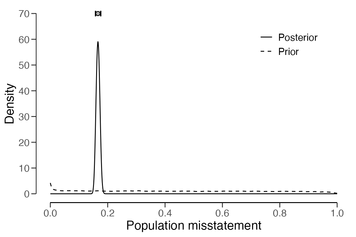
##   20  4000  15  3  3 0.20000 0.07266 0.45646   0.25646

In this scenario, the output of the summary() function indicates that the estimated misstatement in the population is 5.98 percent, with the 95 percent (two-sided) credible interval extending from 4.28 percent to 8.22 percent. The estimates for each stratum vary significantly from one another but exhibit relative uncertainty. They can be visualized via the call below to plot(..., type = "estimates")

plot(result_np, type = "estimates")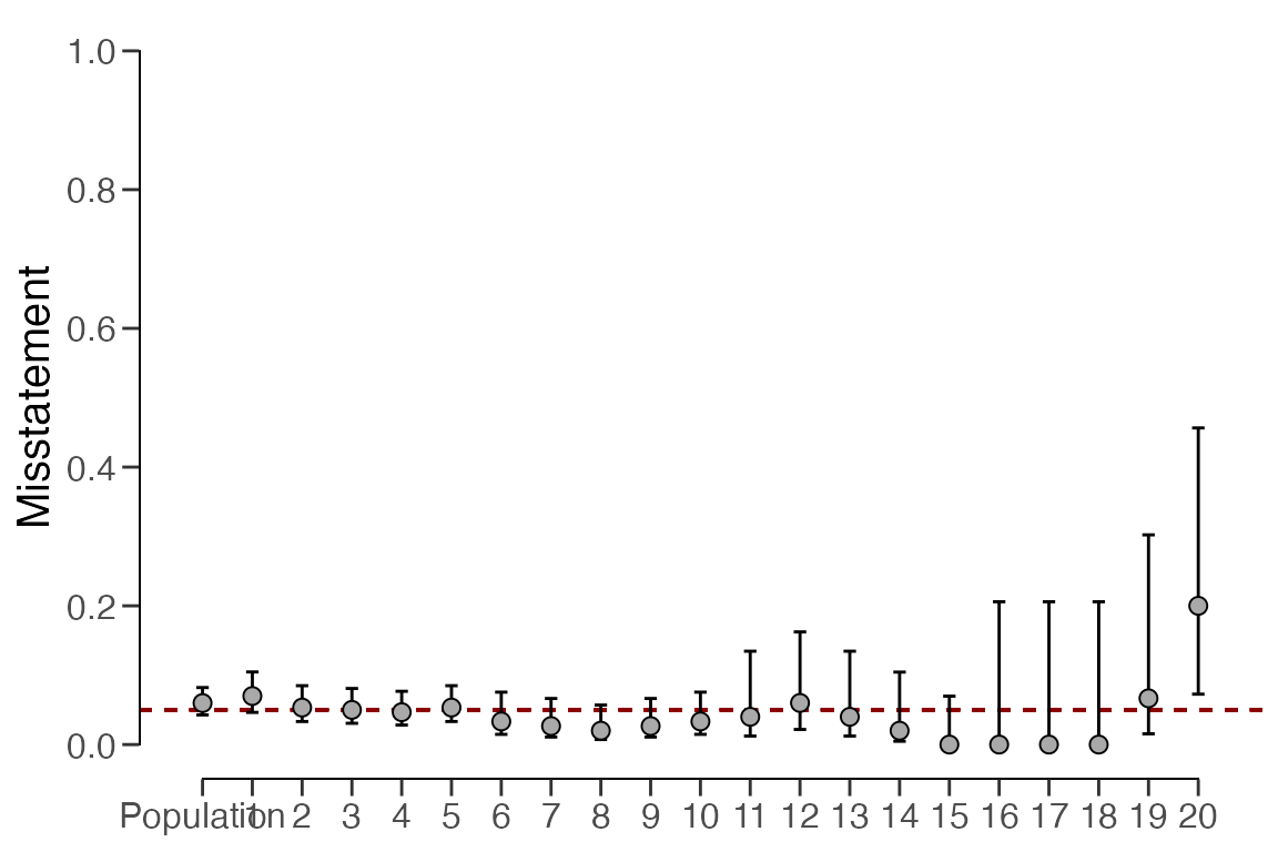

The prior and posterior distribution for the population misstatement can be obtained using the plot(..., type = "posterior") function.

plot(result_np, type = "posterior")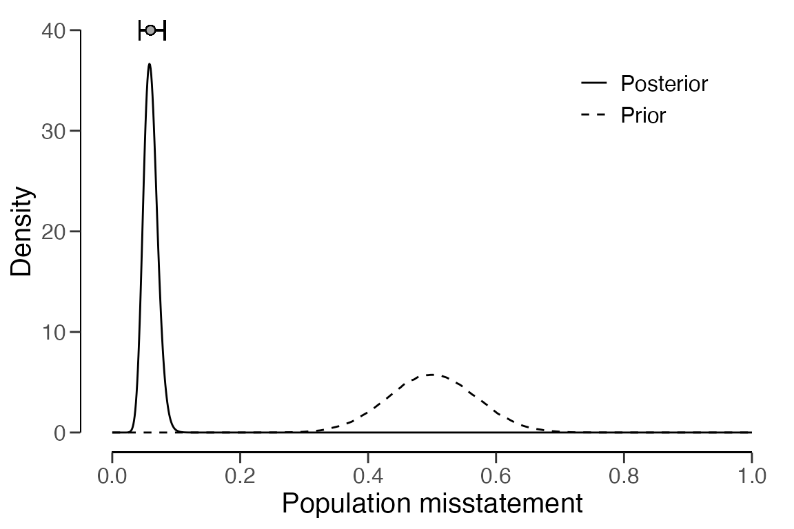

Approach 2: Partial pooling

The partial pooling approach (pooling = "partial") presumes both differences and similarities between strata. This enables the auditor to share information among the strata to minimize uncertainty in the population estimate. The following call evaluates the sample using a Bayesian stratified evaluation procedure, where the stratum estimates are poststratified to derive the population estimate. Remember, it is important to set the seed via set.seed() to make the results reproducible.

set.seed(1)
result_pp <- evaluation(
  materiality = 0.05, method = "binomial",
  n = retailer[["samples"]], x = retailer[["errors"]],
  N.units = retailer[["items"]], pooling = "partial",
  alternative = "two.sided", prior = TRUE
)
summary(result_pp)

## 
##  Bayesian Audit Sample Evaluation Summary
## 
## Options:
##   Confidence level:               0.95 
##   Population size:                144000 
##   Materiality:                    0.05 
##   Hypotheses:                     H₀: Θ = 0.05 vs. H₁: Θ ≠ 0.05 
##   Method:                         binomial 
##   Prior distribution:             Nonparametric 
## 
## Data:
##   Sample size:                    2575 
##   Number of errors:               115 
##   Sum of taints:                  115 
## 
## Results:
##   Posterior distribution:         Nonparametric 
##   Most likely error:              0.0423 
##   95 percent credible interval:   [0.032494, 0.053654] 
##   Precision:                      0.011354 
##   BF₁₀:                            0.030086 
## 
## Strata (20):
##          N   n  x  t    mle      lb      ub precision
##   1   5000 300 21 21 0.0579 0.04003 0.08836   0.03046
##   2   5000 300 16 16 0.0503 0.03217 0.07359   0.02329
##   3   5000 300 15 15 0.0424 0.03042 0.07060   0.02820
##   4   5000 300 14 14 0.0425 0.02849 0.06764   0.02514
##   5   5000 300 16 16 0.0437 0.03195 0.07382   0.03012
##   6   5000 150  5  5 0.0378 0.01823 0.06365   0.02585
##   7   5000 150  4  4 0.0360 0.01511 0.05944   0.02344
##   8   5000 150  3  3 0.0341 0.01177 0.05539   0.02129
##   9   5000 150  4  4 0.0364 0.01474 0.05940   0.02300
##   10  5000 150  5  5 0.0357 0.01783 0.06357   0.02787
##   11 10000  50  2  2 0.0433 0.01658 0.08010   0.03680
##   12 10000  50  3  3 0.0431 0.02147 0.09121   0.04811
##   13 10000  50  2  2 0.0373 0.01676 0.07932   0.04202
##   14 10000  50  1  1 0.0356 0.01120 0.07089   0.03529
##   15 10000  50  0  0 0.0392 0.00548 0.06181   0.02261
##   16 10000  15  0  0 0.0364 0.00895 0.08006   0.04366
##   17 10000  15  0  0 0.0374 0.00861 0.07943   0.04203
##   18 10000  15  0  0 0.0387 0.00867 0.08028   0.04158
##   19 10000  15  1  1 0.0403 0.01598 0.09819   0.05789
##   20  4000  15  3  3 0.0472 0.02772 0.13675   0.08955

In this scenario, the output indicates that the estimated misstatement in the population is 4.23 percent, with the 95 percent credible interval extending from 3.25 percent to 5.37 percent. Note that this population estimate is considerably less uncertain compared to the no pooling approach. Similarly to the no pooling approach, the stratum estimates differ from each other but are closer together and exhibit less uncertainty. This can be explained by the fact that the partial pooling approach allows for information to be shared between strata. The stratum estimates can be visualized via a call to plot(..., type = "estimates").

plot(result_pp, type = "estimates")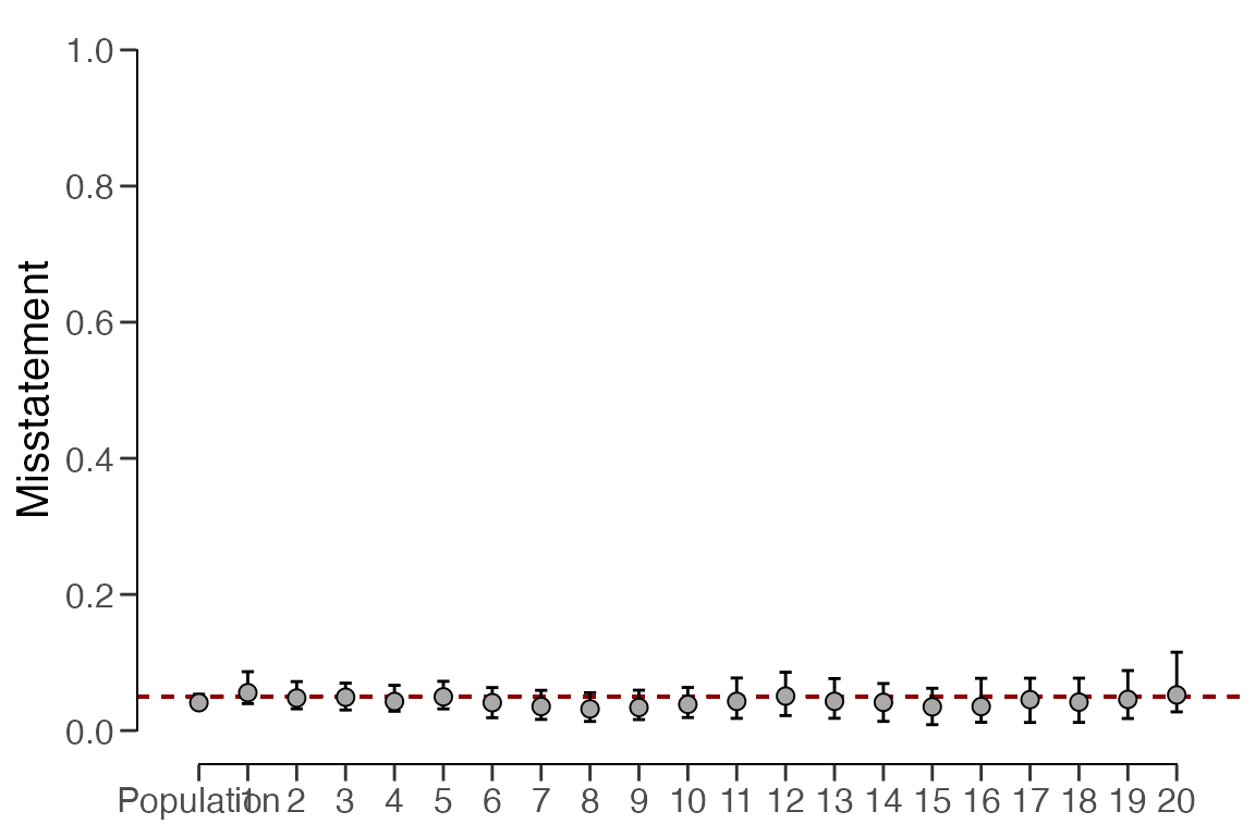

The prior and posterior distribution for the population misstatement can be obtained using the plot(..., type = "posterior") function.

plot(result_pp, type = "posterior")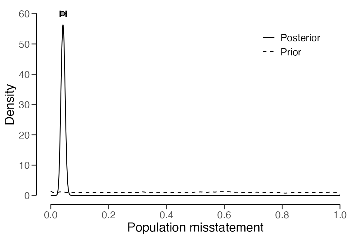

Evaluation using data

We now consider the situation where the auditor has access to the sample (and potentially the population) data and wants to perform inference about the misstatement using these data.

Non-stratified samples

In this example, we will demonstrate how to evaluate a non-stratified sample using a data set. For this, we will use the accounts data that is included in the package. These data represent an audit sample obtained from a population of $N$ = 87 accounts receivable, totaling $612,824 in book value (Higgins & Nandram, 2009; Lohr, 2021).

data("accounts")
head(accounts)

##   account bookValue auditValue
## 1       3      6842       6842
## 2       9     16350      16350
## 3      13      3935       3935
## 4      24      7090       7050
## 5      29      5533       5533
## 6      34      2163       2163

To evaluate a non-stratified sample using data, you need to specify the data, values, and values.audit arguments in the evaluation() function. The input for the latter two arguments should be the name of the corresponding column in the input for the data argument. In the accounts data, these two columns are called bookValue and auditValue, respectively.

Classical approach

The command below evaluates the allowances sample using a classical non-stratified evaluation approach.

evaluation(
  data = accounts, method = "binomial",
  values = "bookValue", values.audit = "auditValue"
)

## 
##  Classical Audit Sample Evaluation
## 
## data:  accounts
## number of errors = 4, number of samples = 20, taint = 0.16127
## 95 percent confidence interval:
##  0.0000000 0.1527346
## most likely estimate:
##  0.0080633 
## results obtained via method 'binomial'

In this instance, the output indicates that the estimated most likely misstatement in the population is 0.81 percent. The 95 percent (one-sided) confidence interval extends from 0 percent to 15.27 percent. More detailed information about the results can be obtained via the summary() function.

Bayesian approach

The call below evaluates the accounts sample using a Bayesian non-stratified evaluation procedure.

result <- evaluation(
  data = accounts, method = "binomial",
  values = "bookValue", values.audit = "auditValue", prior = TRUE
)
print(result)

## 
##  Bayesian Audit Sample Evaluation
## 
## data:  accounts
## number of errors = 4, number of samples = 20, taint = 0.16127
## 95 percent credible interval:
##  0.000000 0.145994
## most likely estimate:
##  0.0080633 
## results obtained via method 'binomial' + 'prior'

The output shows that the estimate of the misstatement in the population is again 0.81 percent, with the 95 percent (one-sided) credible interval ranging from 0 percent to 14.6 percent. For the Bayesian analysis, the prior and posterior distribution can be visualized by a call to plot(..., type = "posterior").

plot(result, type = "posterior")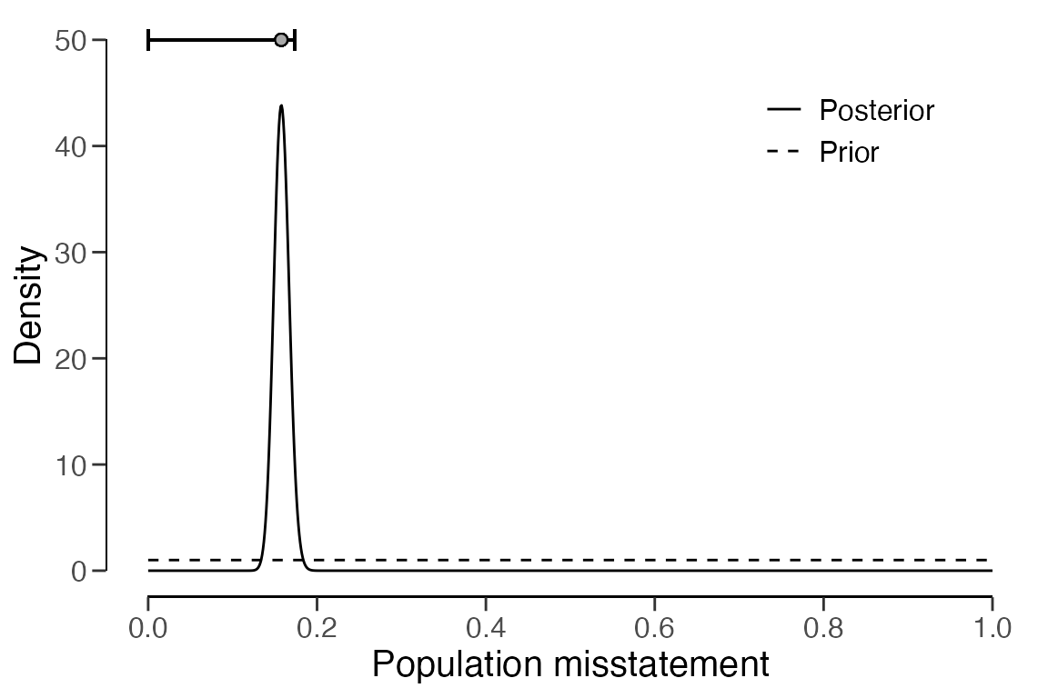

You can also quantify and monitor evidence for or against the claim that the misstatement is lower than a specific performance materiality using the Bayes factor. Suppose that the performance materiality for this example is set to ten percent of the population value. It is recommended to use an impartial prior distribution when calculating the Bayes factor, which can be set up using the code below.

prior <- auditPrior(
  materiality = 0.1, method = "impartial", likelihood = "binomial"
)

After it has been specified, you can use the impartial prior distribution in the evaluation() function as input for the prior argument.

result <- evaluation(
  materiality = 0.1, data = accounts, method = "binomial",
  values = "bookValue", values.audit = "auditValue", prior = prior
)
print(result)

## 
##  Bayesian Audit Sample Evaluation
## 
## data:  accounts
## number of errors = 4, number of samples = 20, taint = 0.16127, BF₁₀ =
## 11.274
## alternative hypothesis: true misstatement rate is less than 0.1
## 95 percent credible interval:
##  0.0000000 0.1171385
## most likely estimate:
##  0.0063047 
## results obtained via method 'binomial' + 'prior'

It can be seen from the output that the Bayes factor in favor of the hypothesis of tolerable misstatement is 11.274. This indicates that the data is roughly 11 times more likely under the hypothesis of tolerable misstatement than under the hypothesis of intolerable misstatement. Besides computing the Bayes factor for the total sample, it is also possible to see how the Bayes factor evolves as a function of the sample size. This can be done via a call to plot(..., type = "sequential").

plot(result, type = "sequential")

Stratified samples

In this example, we will demonstrate how to evaluate a stratified sample using a data set. We will use the allowances data set that is included in the package. This data set comprises $N$ = 3500 subsidy declarations from municipalities. Each line item has a recorded value book value (column bookValue) and an audited value (column auditValue), which is the true value for the purpose of this illustration. The data set already identifies the items that have been audited as part of the sample in the column times. In this scenario, we will only be performing estimation and therefore do not specify the materiality argument in the evaluation() function.

data("allowances")
head(allowances)

##   item branch bookValue auditValue times
## 1    1     12      1600       1600     1
## 2    2     12      1625         NA     0
## 3    3     12      1775         NA     0
## 4    4     12      1250       1250     1
## 5    5     12      1400         NA     0
## 6    6     12      1190         NA     0

To evaluate a stratified sample using a data set, you need to specify the data, values, values.audit, and strata arguments in the evaluation() function. The input for N.units is once again optional. In this example, the units are monetary, determined by summing up the book values of the items within each stratum. For instance, we can see that stratum two is the largest, with a total value of $2,792,814.33 and stratum five is the smallest, with a total value of $96,660.53.

N.units <- aggregate(allowances$bookValue, list(allowances$branch), sum)$x
print(data.frame(N.units))

##       N.units
## 1   317200.09
## 2  2792814.33
## 3  1144231.69
## 4   414202.89
## 5    96660.53
## 6   348006.13
## 7  2384079.33
## 8  1840399.33
## 9   563957.70
## 10 3198877.73
## 11 1983299.06
## 12  319144.13
## 13  148905.79
## 14  513058.76
## 15  432007.61
## 16  275403.70

Classical approach

The following command evaluates the allowances sample using a classical stratified evaluation method. In this process, the estimates from each stratum are poststratified to derive the estimate for the entire population. Note that for computational reasons it is important to set a seed here via set.seed(). Furthermore, note that the sample is automatically separated from the population because the times value for items not in the sample is 0.

set.seed(1)
result <- evaluation(
  data = allowances, times = "times", method = "binomial",
  values = "bookValue", values.audit = "auditValue",
  N.units = N.units, strata = "branch",
  alternative = "two.sided"
)
print(result)

## 
##  Classical Audit Sample Evaluation
## 
## data:  allowances
## number of errors = 401, number of samples = 1604, taint = 252.93
## 95 percent confidence interval:
##  0.1298437 0.1759994
## most likely estimate:
##  0.14723 
## results obtained via method 'binomial' + 'no-pooling'

In this instance, the output reveals that the estimated misstatement in the population is 14.72 percent. The 95 percent confidence interval spans from 12.98 percent to 17.6 percent. The precision of the population estimate is therefore 4.26 percent. The estimates for each stratum are visualized below. For more detailed information, including the actual stratum estimates, you can use the summary() function.

plot(result, type = "estimates")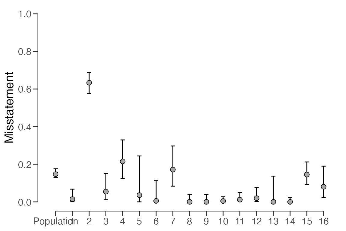

Bayesian approach

Bayesian inference can enhance the estimates obtained from the classical approach by pooling information across strata where feasible. The following command evaluates the allowances sample using a Bayesian stratified evaluation method. In this process, the estimates from each stratum are pooled and poststratified to derive the estimate for the entire population.

set.seed(1)
result <- evaluation(
  data = allowances, times = "times", method = "binomial",
  values = "bookValue", values.audit = "auditValue",
  N.units = N.units, strata = "branch", pooling = "partial",
  alternative = "two.sided",
  prior = TRUE
)
print(result)

## 
##  Bayesian Audit Sample Evaluation
## 
## data:  allowances
## number of errors = 401, number of samples = 1350, taint = 224.66
## 95 percent credible interval:
##  0.1571337 0.1757009
## most likely estimate:
##  0.1659 
## results obtained via method 'binomial' + 'partial-pooling' + 'prior'

The output indicates that the estimated misstatement in the population is 16.59 percent. The 95 percent credible interval spans from 15.71 percent to 17.57 percent. The precision of the population estimate is therefore 1.86 percent, which is lower than that of the classical approach. The estimates for each stratum are visualized below using the plot(..., type = "estimates) command but their actual values can be once again be obtained using the summary() function.

plot(result, type = "estimates")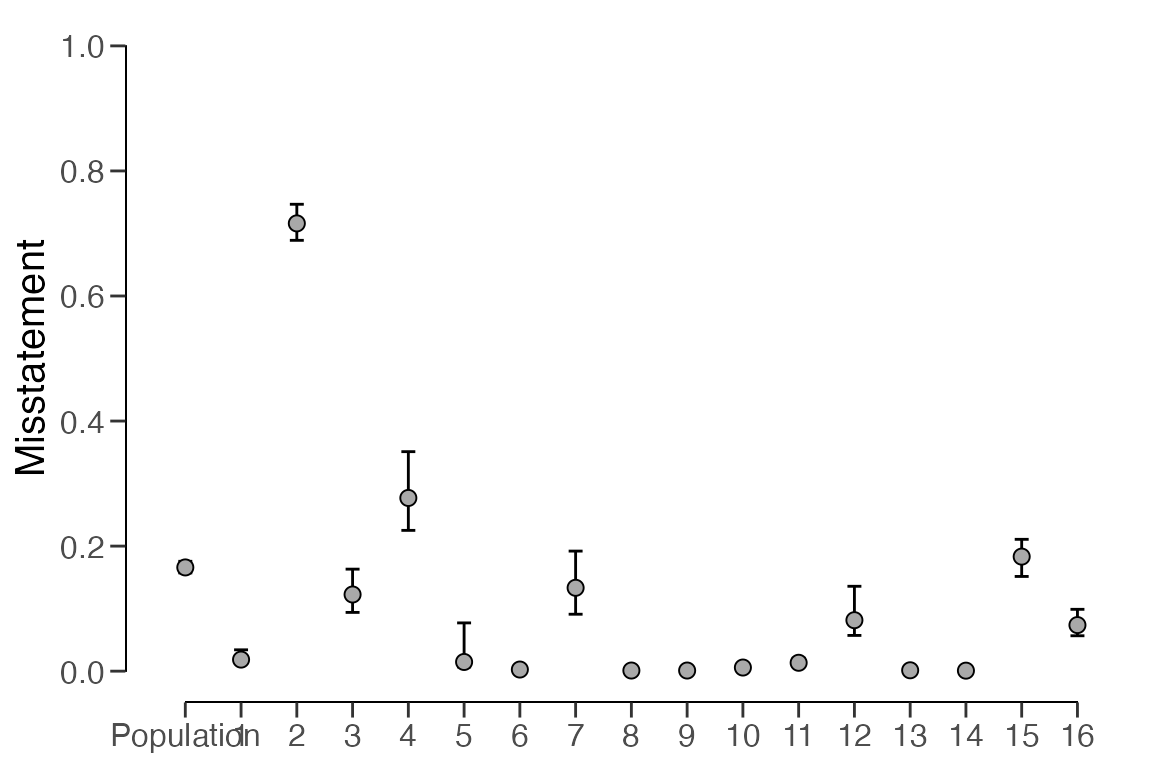

The prior and posterior distribution for the population misstatement can be obtained via the plot(..., type = "posterior") function.

plot(result, type = "posterior")

References

Derks, K., Swart, J. de, Batenburg, P. van, Wagenmakers, E.-J., & Wetzels, R. (2021). Priors in a Bayesian audit: How integration of existing information into the prior distribution can improve audit transparency and efficiency. International Journal of Auditing, 25(3), 621–636. https://doi.org/10.1111/ijau.12240

Derks, K., Swart, J. de, Wagenmakers, E.-J., & Wetzels, R. (2022a). An impartial Bayesian hypothesis test for audit sampling. https://doi.org/10.31234/osf.io/8nf3e

Derks, K., Swart, J. de, Wagenmakers, E.-J., & Wetzels, R. (2022b). Bayesian generalized linear modeling for audit sampling: How to incorporate audit information into the statistical model. PsyArXiv. https://doi.org/10.31234/osf.io/byj2a

Derks, K., Swart, J. de, Wagenmakers, E.-J., & Wetzels, R. (2024). The Bayesian approach to audit evidence: Quantifying statistical evidence using the bayes factor. Auditing: A Journal of Practice & Theory. https://doi.org/10.31234/osf.io/kzqp5

Higgins, H. N., & Nandram, B. (2009). Monetary unit sampling: Improving estimation of the total audit error. Advances in Accounting, 25(2), 174–182. https://doi.org/10.1016/j.adiac.2009.06.001

Lohr, S. L. (2021). Sampling: Design and analysis. Chapman; Hall/CRC. https://doi.org/10.1201/9780429298899

Stewart, T. R. (2012). Technical notes on the AICPA audit guide audit sampling. American Institute of Certified Public Accountants.

Stewart, T. R. (2013). A Bayesian audit assurance model with application to the component materiality problem in group audits [PhD thesis, VU University]. https://hdl.handle.net/1871/39813

Koen Derks

Introduction

Required information

Evaluation using summary statistics

Non-stratified samples

Classical approach

Bayesian approach

Stratified samples

Approach 1: No pooling

Approach 2: Partial pooling

Evaluation using data

Non-stratified samples

Classical approach

Bayesian approach

Stratified samples

Classical approach

Bayesian approach

References