Creating a prior distribution for audit sampling

Koen Derks

Introduction

This vignette will walk you through the process of setting up a prior distribution for audit sampling using the auditPrior() function in the jfa package.

The power of Bayesian statistics lies in its ability to incorporate pre-existing information about the misstatement into the sampling procedure through the prior distribution. Once data is observed, the prior information is updated to draw an overall conclusion about the misstatement in the population. The use of a prior distribution has the advantage of making the underlying assumptions explicit, potentially reducing the amount of audit work needed to achieve the desired assurance. The type of information that can be incorporated into the prior distribution depends on the availability and quality of the information, as well as the specifics of the audit.

For example, if you have information from the auditee’s internal control systems indicating well-segregated duties and numerous effective controls in place, this suggests a relatively low probability of misstatement. This risk-mitigating information can be incorporated into the prior distribution, thereby lessening the need for evidence from the sample. It is important to note that all information integrated into the prior distribution should be substantiated with appropriate and sufficient audit evidence. Specifically, the auditor should be able to justifying the translation of audit information into a prior distribution. This vignette addresses this issue.

Creating a prior distribution

The auditPrior() function is used to define a prior distribution for audit sampling. The following are various ways this function can be used to construct a prior distribution.

Default priors

The default prior distributions in jfa are specified using method = 'default'. These default priors meet two criteria: 1) they hold relatively minimal information about the population misstatement, and 2) they are proper, meaning they integrate to one.

• likelihood = 'poisson': gamma($\alpha$ = 1, $\beta$ = 1)
• likelihood = 'binomial': beta($\alpha$ = 1, $\beta$ = 1)
• likelihood = 'hypergeometric': beta-binomial(N, $\alpha$ = 1, $\beta$ = 1)
• likelihood = 'normal': normal($\mu$ = 0, $\sigma$ = 1000)
• likelihood = 'uniform': uniform(min = 0, max = 1)
• likelihood = 'cauchy': Cauchy($x_0$ = 0, $\gamma$ = 1000)
• likelihood = 't': Student-t(df = 1)
• likelihood = 'chisq': chi-squared(df = 1)
• likelihood = 'exponential': exponential($\lambda$ = 1)

prior <- auditPrior(method = "default", likelihood = "binomial")
summary(prior)

## 
##  Prior Distribution Summary
## 
## Options:
##   Likelihood:                    binomial 
##   Specifics:                     default prior 
## 
## Results:
##   Functional form:               beta(α = 1, β = 1) 
##   Mode:                          NaN 
##   Mean:                          0.5 
##   Median:                        0.5 
##   Variance:                      0.083333 
##   Skewness:                      0 
##   Information entropy (nat):     0 
##   95 percent upper bound:        0.95 
##   Precision:                     NaN

After setting up the prior distribution, you can visually examine it using the plot() function.

plot(prior)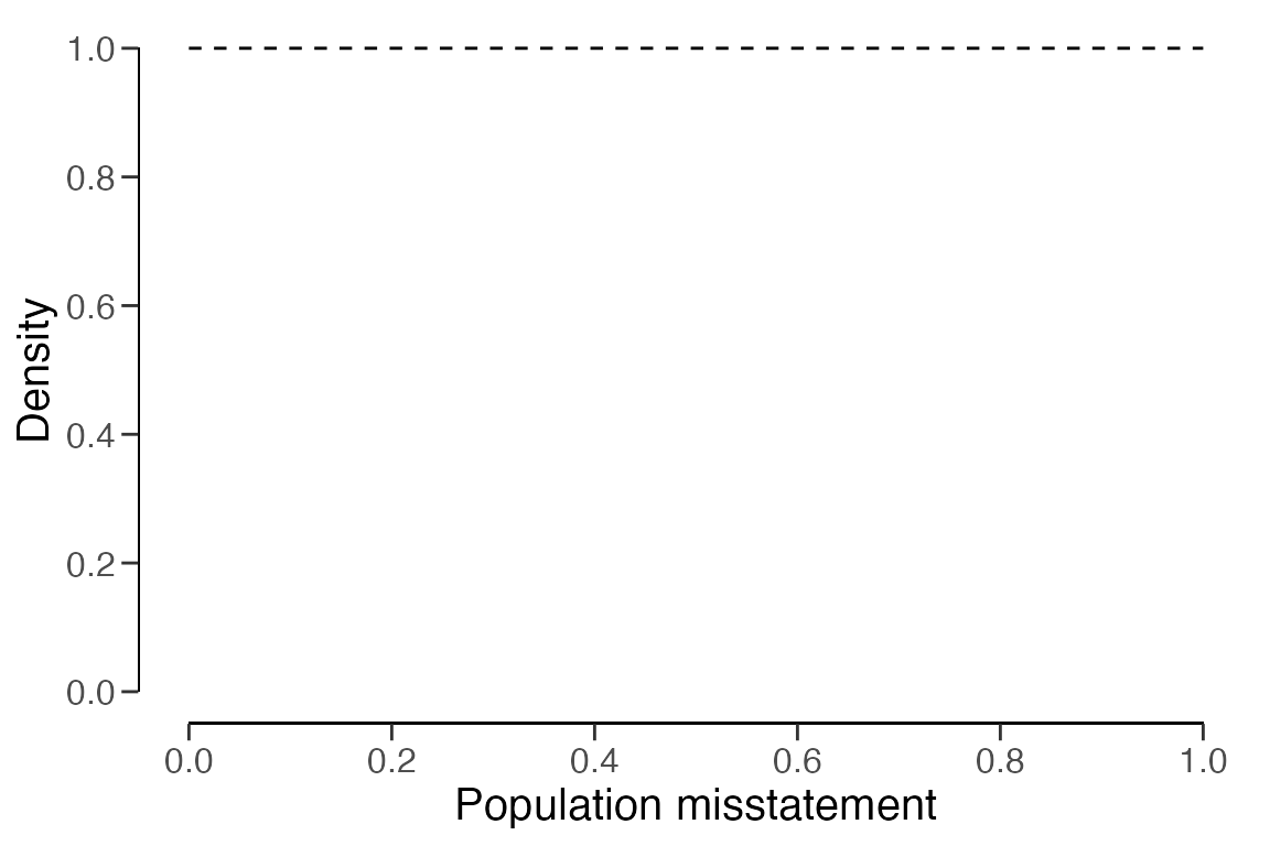

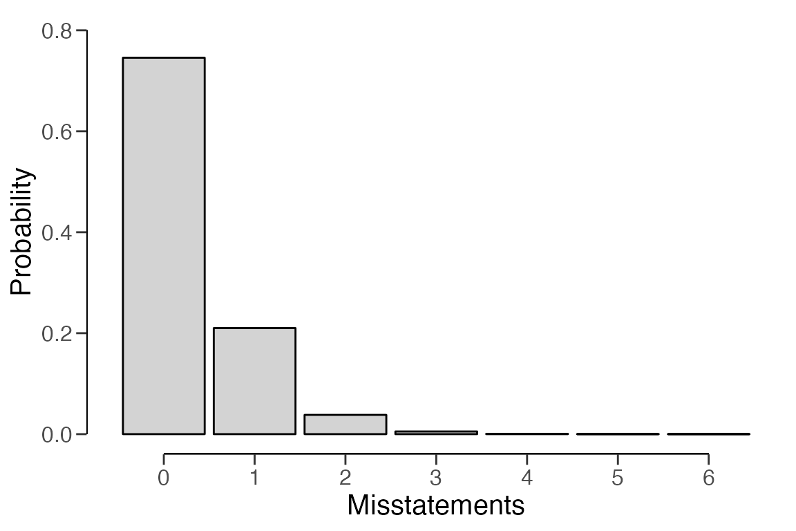
Additionally, the predict() function generates the predictions of the prior distribution at the data level for a sample of $n$ items. For instance, the command below calls for the prediction of the default beta(1, 1) prior for a hypothetical sample of $n$ = 6 items.

predict(prior, n = 6)

##       x=0       x=1       x=2       x=3       x=4       x=5       x=6 
## 0.1428571 0.1428571 0.1428571 0.1428571 0.1428571 0.1428571 0.1428571

You can visualize the predictions of the prior distribution using the plot() function.

plot(predict(prior, n = 10))

Priors with custom parameters

You can manually set the parameters of the prior distribution using method = 'param' along with the alpha and beta arguments. These correspond to the first and (optionally) second parameter of the prior distribution as shown in the default prior section. For instance, the commands below will create a beta(2, 10) prior distribution, a normal(0.025, 0.05) prior distribution, and a Student-t(0.01) prior distribution.

auditPrior(method = "param", likelihood = "binomial", alpha = 2, beta = 10)

## 
##  Prior Distribution for Audit Sampling
## 
## functional form: beta(α = 2, β = 10) 
## parameters obtained via method 'param'

auditPrior(method = "param", likelihood = "normal", alpha = 0.025, beta = 0.05)

## 
##  Prior Distribution for Audit Sampling
## 
## functional form: normal(μ = 0.025, σ = 0.05)T[0,1] 
## parameters obtained via method 'param'

auditPrior(method = "param", likelihood = "t", alpha = 0.01)

## 
##  Prior Distribution for Audit Sampling
## 
## functional form: Student-t(df = 0.01)T[0,1] 
## parameters obtained via method 'param'

Improper priors

An improper prior distribution with classical properties can be constructed using method = 'strict'. The posterior distribution from this prior produces the same results as the classical methodology in terms of sample sizes and upper limits. However, it only becomes proper once a single non-misstated item is present in the sample (Derks et al., 2022). The command below creates an improper beta(1, 0) prior distribution.

Note: This method requires the poisson, binomial, or hypergeometric likelihood.

auditPrior(method = "strict", likelihood = "binomial")

## 
##  Prior Distribution for Audit Sampling
## 
## functional form: beta(α = 1, β = 0) 
## parameters obtained via method 'strict'

Impartial priors

To incorporate the assumption that tolerable misstatement is equally likely as intolerable misstatement (Derks et al., 2022), you can use method = 'impartial'. For instance, the command below generates an impartial beta prior distribution for a performance materiality of five percent.

Note: This method requires a value for the materiality and the poisson, binomial, or hypergeometric likelihood.

auditPrior(method = "impartial", likelihood = "binomial", materiality = 0.05)

## 
##  Prior Distribution for Audit Sampling
## 
## functional form: beta(α = 1, β = 13.513) 
## parameters obtained via method 'impartial'

Priors based on risk of material misstatement

To manually set prior probabilities for the hypothesis of tolerable misstatement and the hypotheses of intolerable misstatement (Derks et al., 2021), you can use method = 'hyp' in conjunction with the p.hmin argument. For instance, the command below integrates the information that the hypothesis of intolerable misstatement has a 40 percent probability into a beta prior distribution. This is equal to setting the risk of material misstatement (RMM) to 40 percent.

Note: This method requires a value for the materiality and the poisson, binomial, or hypergeometric likelihood.

auditPrior(method = "hyp", likelihood = "binomial", materiality = 0.05, p.hmin = 1 - 0.4)

## 
##  Prior Distribution for Audit Sampling
## 
## functional form: beta(α = 1, β = 17.864) 
## parameters obtained via method 'hyp'

Priors based on the Audit Risk Model

To convert risk assessments from the Audit Risk Model, including inherent risk and internal control risk, into a prior distribution (Derks et al., 2021), you can use method = 'arm' along with the ir and cr arguments. For instance, the command below integrates the information that the inherent risk is 90 percent and the internal control risk is 60 percent into a beta prior distribution.

Note: This method requires the poisson, binomial, or hypergeometric likelihood.

auditPrior(method = "arm", likelihood = "binomial", materiality = 0.05, ir = 0.9, cr = 0.6)

## 
##  Prior Distribution for Audit Sampling
## 
## functional form: beta(α = 1, β = 12) 
## parameters obtained via method 'arm'

Priors based on the Bayesian Risk Assessment Model

Incorporating information about the most likely value and the upper limit of the population misstatement can be done using method = 'bram'. For instance, the following code demonstrates how to embed the information that the most likely misstatement in the population is one percent and the 95 percent upper limit on this misstatement is 60 percent into a beta prior distribution.

Note: This method requires the poisson, binomial, or hypergeometric likelihood.

auditPrior(method = "bram", likelihood = "binomial", expected = 0.01, materiality = 0.05, ub = 0.6)

## 
##  Prior Distribution for Audit Sampling
## 
## functional form: beta(α = 1.023, β = 3.317) 
## parameters obtained via method 'bram'

Priors based on an earlier sample

You can use the method = 'sample' along with the x and n arguments to integrate information from an earlier sample into the prior distribution (Derks et al., 2021). For instance, the code below demonstrates how to include the data from a previous sample of $n$ = 30 items where $k$ = 0 misstatements were detected into a beta prior distribution.

Note: This method requires the poisson, binomial, or hypergeometric likelihood.

auditPrior(method = "sample", likelihood = "binomial", x = 0, n = 30)

## 
##  Prior Distribution for Audit Sampling
## 
## functional form: beta(α = 1, β = 30) 
## parameters obtained via method 'sample'

Priors based on a weighted earlier sample

You can integrate information from the previous year’s results, adjusted by a factor (Derks et al., 2021), into the prior distribution using method = 'power' in conjunction with the x and n arguments. For instance, the code below demonstrates how to include the data from the previous year’s results (i.e., a sample of $n$ = 58 items with $k$ = 0 misstatements found), weighed by a factor of 0.7, into a beta prior distribution. This factor delta of 0.7 could be derived from the fact that 70 percent of the auditee’s contracts are with businesses that have remained unchanged over the years, implying that last year’s population is for 70 percent comparable to the population of this year.

Note: This method requires the poisson, binomial, or hypergeometric likelihood.

auditPrior(method = "power", likelihood = "binomial", x = 0, n = 58, delta = 0.7)

## 
##  Prior Distribution for Audit Sampling
## 
## functional form: beta(α = 1, β = 40.6) 
## parameters obtained via method 'power'

Nonparametric prior distributions

You can establish the prior based on samples from the prior distribution using method = 'nonparam' along with the samples argument. For instance, the code below sets up a prior based on 1000 samples from a beta(1, 10) distribution.

Note: The likelihood argument is not required and will be ignored in this method.

auditPrior(method = "nonparam", samples = rbeta(1000, 1, 10))

## 
##  Prior Distribution for Audit Sampling
## 
## functional form: Nonparametric 
## parameters obtained via method 'nonparam'

Using a prior distribution

The objects returned by the auditPrior() function can be used as input for the prior argument in both the planning() and evaluation() functions. Here follows a brief demonstration of how to construct the prior distribution using these functions.

Planning a sample

The prior distribution can be employed during the planning stage to compute a minimum sample size. This is done by supplying the object returned by the auditPrior() function to the planning() function via its prior argument. For instance, the command below calculates the minimum sample size required to test the misstatement in the population against a performance materiality of five percent, using a beta(1, 10) prior distribution. The resulting sample size is $n$ = 49.

prior <- auditPrior(method = "param", likelihood = "binomial", alpha = 1, beta = 10)
planning(materiality = 0.05, likelihood = "binomial", prior = prior)

## 
##  Bayesian Audit Sample Planning
## 
## minimum sample size = 49 
## sample size obtained in 50 iterations via method 'binomial' + 'prior'

Evaluating a sample

The prior distribution can also be used during the evaluation stage by providing the object returned by the auditPrior() function to the evaluation() function via its prior argument. For example, the command below evaluates the misstatement in the population with respect to a performance materiality of five percent after observing a sample of $n$ = 60 items with $k$ = 1 misstatement, using a Normal(0.025, 0.05) prior distribution.

prior <- auditPrior(method = "param", likelihood = "normal", alpha = 0.025, beta = 0.05)
eval <- evaluation(materiality = 0.05, x = 1, n = 60, prior = prior)
summary(eval)

## 
##  Bayesian Audit Sample Evaluation Summary
## 
## Options:
##   Confidence level:               0.95 
##   Materiality:                    0.05 
##   Hypotheses:                     H₀: Θ > 0.05 vs. H₁: Θ < 0.05 
##   Method:                         poisson 
##   Prior distribution:             normal(μ = 0.025, σ = 0.05)T[0,1] 
## 
## Data:
##   Sample size:                    60 
##   Number of errors:               1 
##   Sum of taints:                  1 
## 
## Results:
##   Posterior distribution:         Nonparametric 
##   Most likely error:              0.018 
##   95 percent credible interval:   [0, 0.066] 
##   Precision:                      0.048 
##   BF₁₀:                            4.8232

The prior and posterior distribution can be visualized by calling plot(..., type = "posterior").

plot(eval, type = "posterior")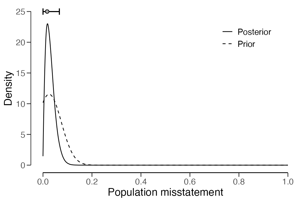

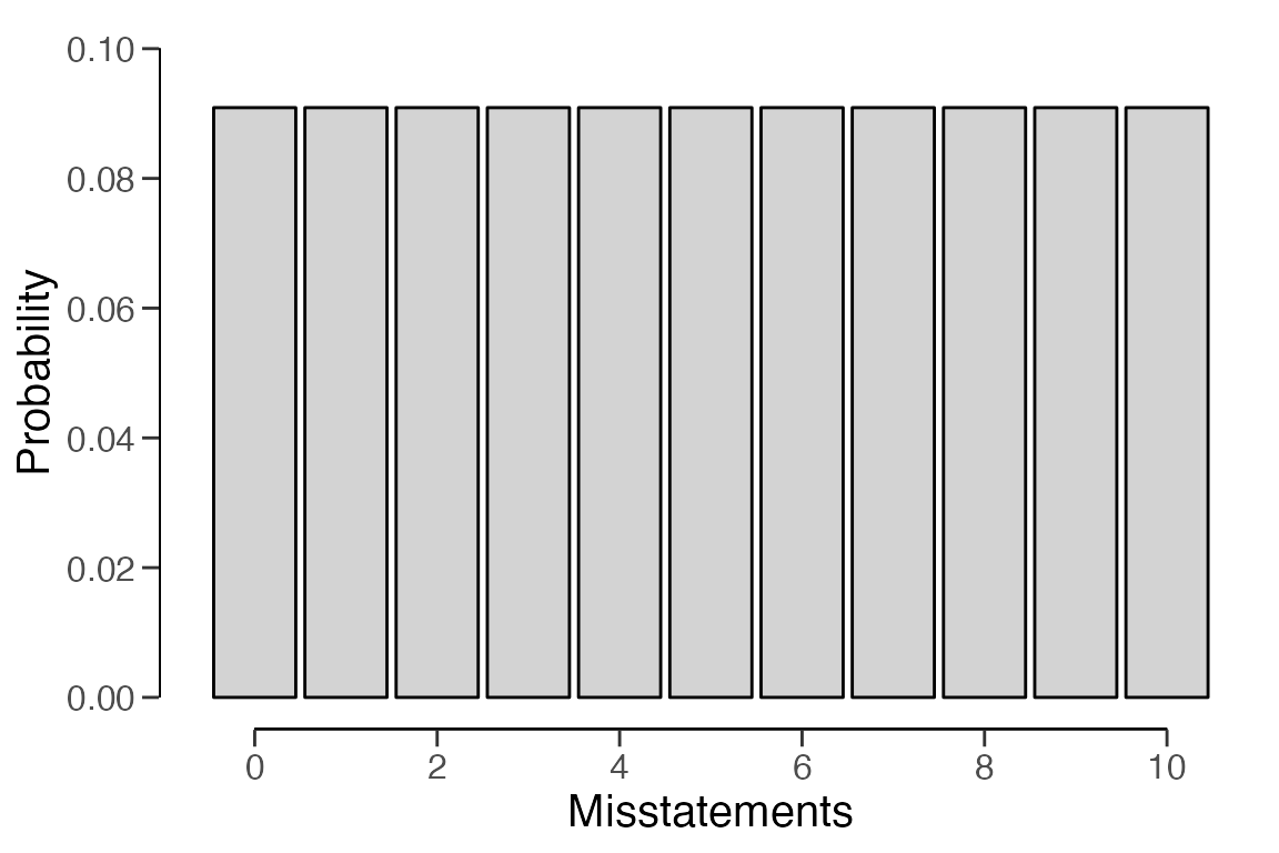
Furthermore, the predictions of the posterior distribution at the data level can be visualized by combining the predict() and plot() functions. For instance, the command below displays the predictions of the posterior distribution for a hypothetical (next) sample of $n$ = 10 items.

plot(predict(eval$posterior, n = 10))

References

Derks, K., Swart, J. de, Batenburg, P. van, Wagenmakers, E.-J., & Wetzels, R. (2021). Priors in a Bayesian audit: How integration of existing information into the prior distribution can improve audit transparency and efficiency. International Journal of Auditing, 25(3), 621–636. https://doi.org/10.1111/ijau.12240

Derks, K., Swart, J. de, Wagenmakers, E.-J., & Wetzels, R. (2022). An impartial Bayesian hypothesis test for audit sampling. https://doi.org/10.31234/osf.io/8nf3e