Selecting statistical audit samples
Koen Derks
Source:vignettes/articles/sample-selection.Rmd
sample-selection.RmdIntroduction
Welcome to the ‘Selecting statistical audit samples’ vignette of the
jfa package. This page outlines the most commonly used
sampling methodology for auditing and demonstrates how to select a
sample using these techniques via the selection() function
in the package.

Auditors often need to evaluate balances or processes that involve a large number of items or units. As it is not feasible to individually inspect all of these items or units, they must select a subset (i.e., a sample) from the population to make a statement about a specific characteristic (often the misstatement) of the population. Various sampling methods, which have become standard practice in the field of auditing, are available for this purpose (Leslie et al., 1979).
Sampling units
Selecting a subset of items or units from the population requires knowledge of the sampling units, which are physical representations of the population that needs to be audited. Typically, the auditor must decide between two types of sampling units: individual items in the population or individual monetary units in the population. To conduct statistical selection, the population must be segmented into individual sampling units, each of which can be assigned a probability of being included in the sample. The complete collection of all sampling units assigned a selection probability is known as the sampling frame.
Items
A sampling unit for record (i.e., attributes) sampling is usually a characteristic of an item in the population. For instance, if you are inspecting a population of receipts, a potential sampling unit for record sampling could be the date of payment of the receipt. When a sampling unit (e.g., date of payment) is indicated by the sampling method, the population item corresponding to the sampled unit is included in the sample.
Monetary units
A sampling unit for monetary unit sampling differs from a sampling unit for record sampling in that it is an individual monetary unit within an item or transaction, like an individual dollar. For example, a single sampling unit could be the 10 dollar from a specific receipt in the population. When a sampling unit (e.g., individual dollar) is indicated by the sampling method, the population item containing the sampling unit is included in the sample.
Sampling methods
This section discusses the four sampling methods implemented in jfa. First, for notation, let the the population be defined as the total set of individual sampling units: . In statistical sampling, every sampling unit in the population must receive a selection probability .
The purpose of the sampling method is to provide a framework to
assign selection probabilities
to each of the sampling units, and subsequently draw sampling units from
the population until a set of size
has been created. To illustrate the outcomes of different sampling
methods on the same data set, we will use the BuildIt data
set that is included in the package. This data set can be loaded via the
command below.
##      ID bookValue auditValue
## 1 82884    242.61     242.61
## 2 25064    642.99     642.99
## 3 81235    628.53     628.53
## 4 71769    431.87     431.87
## 5 55080    620.88     620.88
## 6 93224    501.76     501.76
Fixed interval sampling
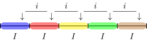
Fixed interval sampling (a.k.a. systematic sampling) is a method designed to generate representative samples from monetary populations. This algorithm establishes a uniform interval on the sampling units. Following this, a starting point is either manually chosen or randomly selected within the first interval. A sampling unit is then selected at each of the uniform intervals from this starting point throughout the population, see Figure 1.
The number of required intervals
can be calculated by dividing the total number of sampling units in the
population
by the desired sample size
:
=
.
For example, if the total population consists of
= 1000 units and the desired sample size is
= 100 units, the interval would be
= 10 sampling units wide. If, subsequently, the
5
sampling unit is chosen as the starting point in the first interval, the
sampling units 5, 15, 25, etc., are selected to be included in the
sample. It is important to note that this selection is entirely
deterministic and depends on the chosen starting point (specified via
start).
The fixed interval method provides a sample where each sampling unit in the population has an equal chance of being selected. However, this method ensures that all items in the population with a monetary value larger than the interval width are always included in the sample, as one of these items’ sampling units will always be selected from the interval. If the population is randomly arranged with respect to its deviation pattern, fixed interval sampling is equivalent to random selection.
Advantage(s): The fixed interval sampling method is often easy to understand and quick to execute. In monetary unit sampling, all items larger than the calculated interval are included in the sample. In record sampling, since units can be ranked based on value, there is a guarantee that some large items will be included in the sample.
Disadvantage(s): A pattern in the population may align with the selected interval, making the sample less representative. An additional complication with this method is that it is difficult to extend the sample after the initial sample has been drawn due to the possibility of selecting the same sampling unit. However, this problem can be efficiently solved by removing the already selected sampling units from the population and redrawing the intervals.
The code below demonstrates how to apply the fixed interval sampling
method in both a record sampling and a monetary unit sampling setting.
By default, the first sampling unit from each interval is selected.
However, this can be changed by setting the argument
start = 1 to a different value.
# Record sampling
result <- selection(
  data = BuildIt, size = 100,
  units = "items", method = "interval", start = 1
)
head(result[["sample"]])
## row times ID bookValue auditValue
## 1 1 1 82884 242.61 242.61
## 2 36 1 80125 118.58 118.58
## 3 71 1 27566 481.44 481.44
## 4 106 1 88261 266.66 266.66
## 5 141 1 58999 568.60 568.60
## 6 176 1 27801 314.65 314.65
# Monetary unit sampling
result <- selection(
  data = BuildIt, size = 100,
  units = "values", method = "interval", values = "bookValue", start = 1
)
head(result[["sample"]])
## row times ID bookValue auditValue
## 1 1 1 82884 242.61 242.61
## 2 38 1 57172 329.30 329.30
## 3 73 1 90160 205.69 205.69
## 4 110 1 4756 295.96 295.96
## 5 146 1 90183 333.28 333.28
## 6 183 1 96080 449.07 449.07Cell sampling
The cell sampling method splits the population into the same set of intervals used by fixed interval sampling. However, unlike fixed interval sampling, a sampling unit is selected within each interval by randomly drawing a number between 1 and the interval range . This results in a variable space between the sampling units, as shown in Figure 2.
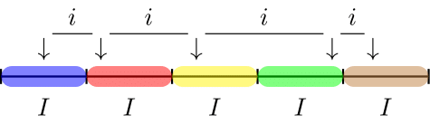
This method ensures that all items in the population with a monetary value larger than twice the interval are always included in the sample, as one of these items’ sampling units will always be selected from one of the two intervals.
Advantage(s): Unlike fixed interval sampling, which has a systematic interval to determine selections, cell sampling allows for more possible sets of samples. It is argued that the cell sampling algorithm addresses the pattern problem found in fixed interval sampling.
Disadvantage(s): Cell sampling has a drawback in that not all items in the population with a monetary value larger than the interval are always included in the sample. Additionally, population items can be located in two adjacent intervals, creating the possibility of an item being included in the sample twice.
The code below demonstrates how to apply the cell sampling method in
both a record sampling and a monetary unit sampling setting. Since this
algorithm involves random number generation, it is important to set a
seed via set.seed() to ensure the results are
reproducible.
# Record sampling
set.seed(1)
result <- selection(
  data = BuildIt, size = 100,
  units = "items", method = "cell"
)
head(result[["sample"]])
## row times ID bookValue auditValue
## 1 9 1 14608 216.48 216.48
## 2 48 1 45437 347.94 139.18
## 3 90 1 90333 241.17 241.17
## 4 136 1 45746 440.72 440.72
## 5 147 1 72906 677.62 677.62
## 6 206 1 93529 528.79 528.79
# Monetary unit sampling
set.seed(1)
result <- selection(
  data = BuildIt, size = 100,
  units = "values", method = "cell", values = "bookValue"
)
head(result[["sample"]])
## row times ID bookValue auditValue
## 1 8 1 81460 295.20 295.20
## 2 53 1 80645 677.88 677.88
## 3 92 1 75133 355.16 355.16
## 4 142 1 68676 612.46 612.46
## 5 153 1 63777 552.83 552.83
## 6 214 1 25379 1021.07 1021.07Random sampling
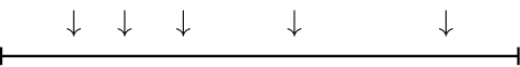
Random sampling is the simplest and most straightforward selection method. This method allows every sampling unit in the population an equal chance of being selected, meaning that every combination of sampling units has the same probability of being selected as every other combination of the same number of sampling units. In essence, the algorithm draws a random selection of size from the sampling units, as illustrated in Figure 3.
Advantage(s): The random sampling method produces an optimal random selection, with the added benefit that the sample can be easily extended by reapplying the same method.
Disadvantages: Since the selection probabilities are equal for all sampling units, there is no guarantee that items in the population with a large monetary value will be included in the sample.
The code below demonstrates how to apply the random sampling method
(with or without replacement using replace) in both a
record sampling and a monetary unit sampling setting. Since this
algorithm involves random number generation, it is important to set a
seed via set.seed() to ensure the results are
reproducible.
# Record sampling
set.seed(1)
result <- selection(
  data = BuildIt, size = 100,
  units = "items", method = "random"
)
head(result[["sample"]])
## row times ID bookValue auditValue
## 1 1017 1 50755 618.24 618.24
## 2 679 1 20237 669.75 669.75
## 3 2177 1 9517 454.02 454.02
## 4 930 1 85674 257.82 257.82
## 5 1533 1 31051 308.53 308.53
## 6 471 1 84375 824.66 824.66
# Monetary unit sampling
set.seed(1)
result <- selection(
  data = BuildIt, size = 100,
  units = "values", method = "random", values = "bookValue"
)
head(result[["sample"]])
## row times ID bookValue auditValue
## 1 1017 1 50755 618.24 618.24
## 2 679 1 20237 669.75 669.75
## 3 2856 1 21836 820.86 820.86
## 4 471 1 84375 824.66 824.66
## 5 270 1 82033 352.75 352.75
## 6 2642 1 49666 601.71 601.71Modified sieve sampling
The fourth and final sampling method option is modified sieve sampling (Hoogduin et al., 2010). This algorithm begins by selecting a standard uniform random number between 0 and 1 for each item in the population. Then, the sieve ratio = is calculated for each item by dividing the book value of the item by the random number. Finally, the items in the population are sorted by their sieve ratio in descending order, and the top items are chosen to be included in the sample. Unlike the classical sieve sampling method (Rietveld, 1978), the modified sieve sampling method allows for precise control over sample sizes.
The code below demonstrates how to apply the modified sieve sampling
method in a monetary unit sampling setting. Since this algorithm
involves random number generation, it is important to set a seed via
set.seed() to ensure the results are reproducible. Also
note that since this algorithm requires the book values of the items, it
is not possible to apply in a record sampling setting.
# Monetary unit sampling
set.seed(1)
result <- selection(
  data = BuildIt, size = 100,
  units = "values", method = "sieve", values = "bookValue"
)
head(result[["sample"]])
## row times ID bookValue auditValue
## 1 2329 1 29919 681.10 681.10
## 2 2883 1 59402 279.29 279.29
## 3 1949 1 56012 581.22 581.22
## 4 3065 1 47482 621.73 621.73
## 5 1072 1 79901 789.97 789.97
## 6 488 1 50811 651.35 651.35Ordering or randomizing the population
The selection() function offers additional arguments
(order, decreasing, and
randomize) that enable you to preprocess your population
before selection. The order argument takes the name of a
column in data as input, and the function then sorts the
population based on this column. The decreasing argument
specifies whether the population is sorted from lowest to highest (when
decreasing = FALSE) or from highest to lowest (when
decreasing = TRUE).
For instance, if you wish to sort the population from the lowest to
the highest book value (found in the bookValue column)
before starting monetary unit sampling, you should use
order = "bookValue" along with the
decreasing = FALSE argument.
set.seed(1)
result <- selection(
  data = BuildIt, size = 100,
  units = "values", values = "bookValue",
  order = "bookValue", decreasing = FALSE
)
head(result[["sample"]])
## row times ID bookValue auditValue
## 1 2662 1 30568 14.47 14.47
## 2 2923 1 63567 125.21 125.21
## 3 2542 1 95807 153.56 153.56
## 4 101 1 64282 172.65 172.65
## 5 838 1 43352 188.72 188.72
## 6 302 1 94296 198.59 198.59In addition, the randomize = TRUE argument can be used
to randomly shuffle the items in the population before selection. By
default, no randomization is applied.
set.seed(1)
result <- selection(
  data = BuildIt, size = 100,
  units = "values", values = "bookValue", randomize = TRUE
)
head(result[["sample"]])
## row times ID bookValue auditValue
## 1 1017 1 50755 618.24 618.24
## 2 2159 1 3653 492.39 492.39
## 3 1639 1 39570 307.54 307.54
## 4 2698 1 225 507.18 507.18
## 5 355 1 27934 749.38 749.38
## 6 1242 1 64071 759.34 759.34