Digit analysis

Koen Derks

Introduction

Welcome to the ‘Digit analysis’ vignette of the jfa package. This page provides comprehensive examples of how to use the digit_test() and repeated_test() functions included in the package.

Function: digit_test()

The digit_test() function accepts a vector of numeric values, extracts the requested digits, and compares the frequencies of these digits to a reference distribution. By default, the function performs a frequentist hypothesis test of the null hypothesis that the digits are distributed according to the reference distribution, and produces a p-value. When a prior is specified, the function performs a Bayesian hypothesis test of the null hypothesis that the digits are distributed according to the reference distribution against the alternative hypothesis that the digits are not distributed according to the reference distribution, and produces a Bayes factor (Kass & Raftery, 1995).

Practical example:

Benford’s law (Benford, 1938) is a principle that describes a pattern in many naturally-occurring numbers. According to Benford’s law, each possible leading digit $d$ in a naturally occurring, or non-manipulated, set of numbers occurs with a probability:

$$\begin{equation} p(d_i) = \text{log}_{10}(1 + \frac{1}{d_i}) \end{equation}$$

The distribution of leading digits in a data set of financial transaction values (e.g., the sinoForest data) can be extracted and tested against the expected frequencies under Benford’s law using the code below.

x <- digit_test(sinoForest$value, check = "first", reference = "benford")
print(x)

## 
##  Classical Digit Distribution Test
## 
## data:  sinoForest$value
## n = 772, MAD = 0.0065981, X-squared = 7.6517, df = 8, p-value = 0.4682
## alternative hypothesis: leading digit(s) are not distributed according to the benford distribution.

You can visually compare the distribution of first digits to the reference distribution by calling plot(..., type = "estimates") on the returned object.

plot(x, type = "estimates")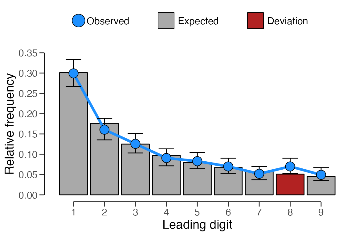

You can also conduct this analysis in a Bayesian manner by setting prior = TRUE, or by providing a value for the prior concentration parameter (e.g., prior = 3).

x <- digit_test(sinoForest$value, check = "first", reference = "benford", prior = TRUE)
print(x)

## 
##  Bayesian Digit Distribution Test
## 
## data:  sinoForest$value
## n = 772, MAD = 0.0065981, BF₁₀ = 1.4493e-07
## alternative hypothesis: leading digit(s) are not distributed according to the benford distribution.

When performing the analysis in a Bayesian manner, you can invoke plot(..., type = "robustness") to assess the robustness of the Bayes factor to the choice of the prior distribution. This will display the Bayes factor under various reasonable specifications of the prior distribution.

plot(x, type = "robustness")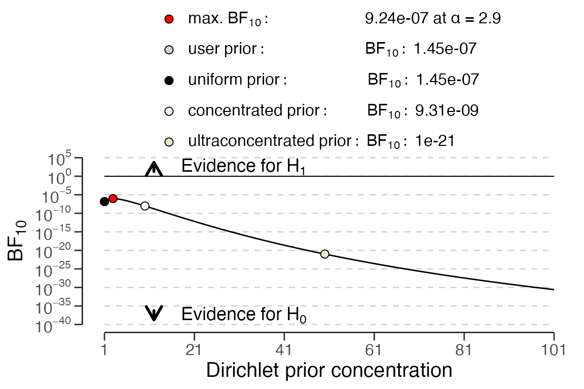

In addition, you can perform a sequential analysis using the Bayes factor by invoking plot(..., type = "sequential"). This sequential analysis includes a robustness check as well.

plot(x, type = "sequential")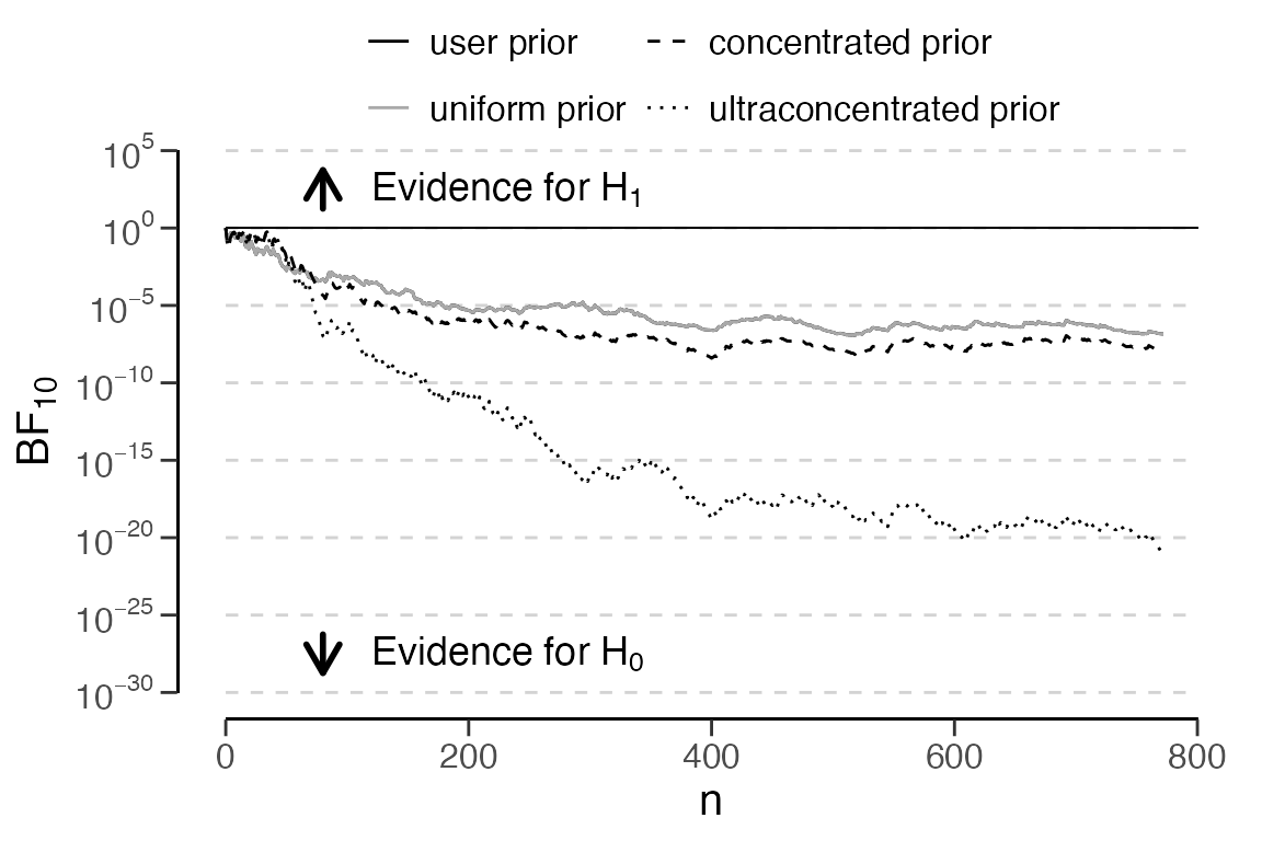

Function: repeated_test()

The repeated_test() function analyzes the frequency with which values are repeated within a set of numbers. Unlike Benford’s law, and its generalizations, this approach examines the entire number at once, not only the first or last digit. For the technical details of this procedure, see (Simonsohn, 2019).

Practical example:

In this example, we analyze a data set from a (retracted) paper that describes three experiments run in Chinese factories, where workers were nudged to use more hand-sanitizer. These data were shown to exhibit two classic markers of data tampering: impossibly similar means and the uneven distribution of last digits (Yu et al., 2018). We can use the repeated_test() function to test if these data also contain a greater amount of repeated values than expected if the data were not tampered with.

x <- repeated_test(sanitizer$value, check = "lasttwo", samples = 2000)
print(x)

## 
##  Classical Repeated Values Test
## 
## data:  sanitizer$value
## n = 1600, AF = 1.5225, p-value = 0.0035
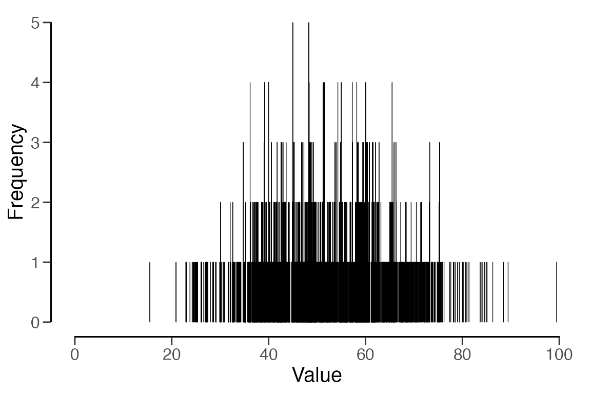
## alternative hypothesis: average frequency in data is greater than for random data.

A histogram of the frequency of each value can be obtained via the plot() function.

plot(x)

References

Benford, F. (1938). The law of anomalous numbers. Proceedings of the American Philosophical Society, 78, 551–572. https://www.jstor.org/stable/984802

Kass, R. E., & Raftery, A. E. (1995). Bayes factors. Journal of the American Statistical Association, 90(430), 773–795. https://doi.org/10.1080/01621459.1995.10476572

Simonsohn, U. (2019). Number-bunching: A new tool for forensic data analysis. https://datacolada.org/77

Yu, F., Nelson, L., & Simonsohn, U. (2018). In press at psychological science: A new ’nudge’ supported by implausible data. https://datacolada.org/74